Code
1library(plotly)- 1
- For interactive plots in the HTML version.
1library(plotly)Real-world data rarely comes as a single series. Sales, tourism demand, energy consumption, and public health metrics are all naturally organized into hierarchies or groups. Forecasting these structures naively — one series at a time — leads to numbers that don’t add up.
Three structures to understand before forecasting them properly.
In a hierarchical structure, every series at a lower level belongs to exactly one series at the level above. The structure is a unique tree.
graph TD
    MX["Mexico (Total)"]
    OAX["Oaxaca"]
    JAL["Jalisco"]
    ETC["···"]
    OJ["Oaxaca City"]
    MH["Miahuatlán"]
    GDL["Guadalajara"]
    TQ["Tequila"]

    MX --> OAX
    MX --> JAL
    MX --> ETC
    OAX --> OJ
    OAX --> MH
    JAL --> GDL
    JAL --> TQ
graph TD
MX["Mexico (Total)"]
OAX["Oaxaca"]
JAL["Jalisco"]
ETC["···"]
OJ["Oaxaca City"]
MH["Miahuatlán"]
GDL["Guadalajara"]
TQ["Tequila"]
MX --> OAX
MX --> JAL
MX --> ETC
OAX --> OJ
OAX --> MH
JAL --> GDL
JAL --> TQ
In a grouped structure, the same set of series can be disaggregated by more than one attribute, none of which nests inside the other.
graph LR
    T["Total Sales"]
    M["Mezcal"]
    TQ["Tequila"]
    B["Brandy"]
    E["···"]

    T --> M
    T --> TQ
    T --> B
    T --> E
graph LR
T["Total Sales"]
M["Mezcal"]
TQ["Tequila"]
B["Brandy"]
E["···"]
T --> M
T --> TQ
T --> B
T --> E
graph LR
    T["Total Sales"]
    R["Retail"]
    BR["Bars & Restaurants"]
    EX["Exports"]

    T --> R
    T --> BR
    T --> EX
graph LR
T["Total Sales"]
R["Retail"]
BR["Bars & Restaurants"]
EX["Exports"]
T --> R
T --> BR
T --> EX
Both diagrams represent the same total sales. A bottle of mezcal sold in retail is simultaneously in the “Mezcal” group and the “Retail” group. There is no single unique tree.
A mixed structure combines a geographic hierarchy (Mexico → State → City) with a grouping attribute (Product type). The most granular series live at the intersection of the hierarchy path and the grouping value.
graph TD
    T["Mexico (Total)"]
    OAX["Oaxaca"]
    JAL["Jalisco"]
    ETC["···"]
    OJ["Oaxaca City × {Mezcal, Tequila, Brandy}"]
    MH["Miahuatlán × {Mezcal, Tequila, Brandy}"]
    GDL["Guadalajara × {Mezcal, Tequila, Brandy}"]
    TQ_["Tequila × {Mezcal, Tequila, Brandy}"]

    T --> OAX
    T --> JAL
    T --> ETC
    OAX --> OJ
    OAX --> MH
    JAL --> GDL
    JAL --> TQ_
graph TD
T["Mexico (Total)"]
OAX["Oaxaca"]
JAL["Jalisco"]
ETC["···"]
OJ["Oaxaca City × {Mezcal, Tequila, Brandy}"]
MH["Miahuatlán × {Mezcal, Tequila, Brandy}"]
GDL["Guadalajara × {Mezcal, Tequila, Brandy}"]
TQ_["Tequila × {Mezcal, Tequila, Brandy}"]
T --> OAX
T --> JAL
T --> ETC
OAX --> OJ
OAX --> MH
JAL --> GDL
JAL --> TQ_
The fpp3 ecosystem (specifically fabletools) provides aggregate_key() to define hierarchical and grouped structures directly on a tsibble.
The tourism dataset — quarterly domestic travel in Australia disaggregated by State, Region, and Purpose — is the canonical example in FPP3 Chapter 11.
tourismaggregate_key(): Defining the StructureA pure hierarchy uses / to denote nesting. A grouped or mixed structure uses * to cross attributes.
tourism_hts <- tourism |>
1  aggregate_key(State / Region, Trips = sum(Trips))

tourism_htsState / Region means Region is nested within State. All aggregations — State totals and the national total — are computed and appended automatically.
tourism_full <- tourism |>
1 aggregate_key(State / Region * Purpose, Trips = sum(Trips))* Purpose crosses the hierarchy with the Purpose grouping. The result includes every combination of (State, Region, Purpose) plus all marginal and total aggregations.
autoplot() on an aggregated tsibble works as usual. Use filter() with is_aggregated() to select a specific level.
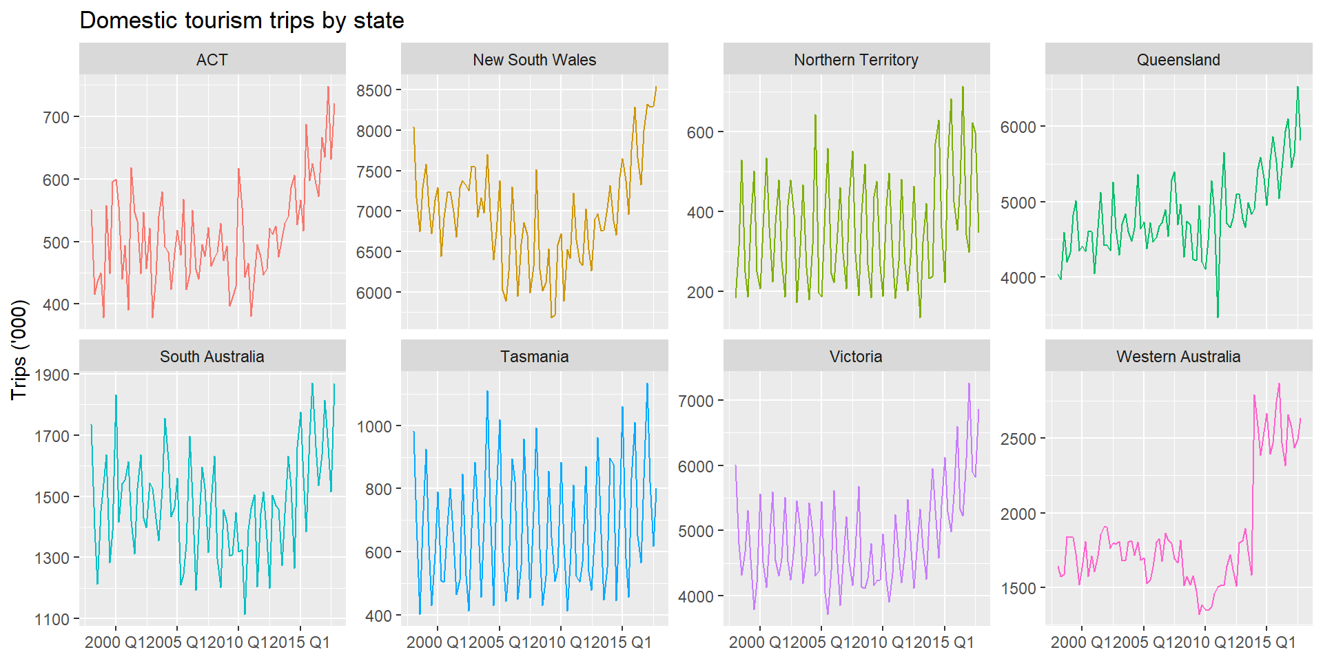
is_aggregated()is_aggregated() returns TRUE for the synthetic aggregation rows created by aggregate_key(). Use it inside filter() to navigate any level of the hierarchy.
tourism_hts |>
1 filter(is_aggregated(State), is_aggregated(Region))tourism_hts |>
1 filter(!is_aggregated(State), is_aggregated(Region))tourism_hts |>
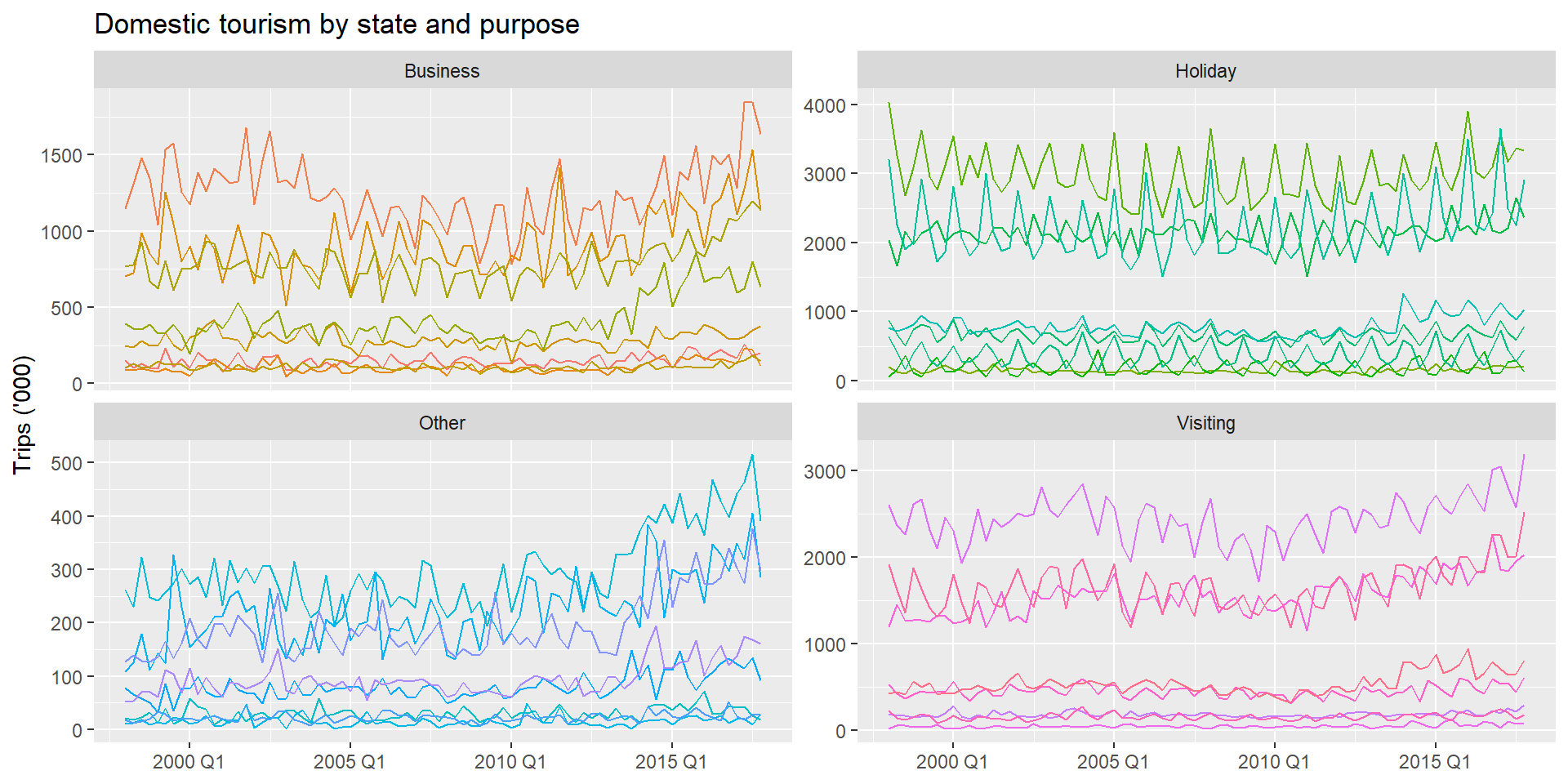
1 filter(!is_aggregated(State), !is_aggregated(Region))With tourism_full, the Purpose grouping is crossed with the State/Region hierarchy:
A set of forecasts is coherent if every aggregate-level forecast equals the sum of its component forecasts.
If \hat{y}_{NSW} and \hat{y}_{VIC} are state-level forecasts, then the national forecast must satisfy \hat{y}_{Total} = \hat{y}_{NSW} + \hat{y}_{VIC} + \cdots
Why does this matter? If you give a retailer a national forecast of 1,000 units and regional forecasts that sum to 850, purchasing, logistics, and budgeting decisions made at different levels of the organization will not align.
Fitting a model independently to every series — including the aggregated ones — almost never produces coherent forecasts.
incoherent_fit <- tourism_hts |>
  filter_index(. ~ "2015 Q4") |>
  model(ets = ETS(Trips))

incoherent_fit |>
  forecast(h = 4) |>
  filter(Quarter == yearquarter("2016 Q1")) |>
  filter(
    is_aggregated(State) |
    (!is_aggregated(State) & is_aggregated(Region))
  ) |>
  as_tibble() |>
  select(State, Region, .mean) |>
  mutate(State = as.character(State), Region = as.character(Region))
The national ETS forecast will not equal the sum of the state ETS forecasts. This is the incoherence problem that reconciliation methods solve.
Single-level approaches fix the coherence problem by choosing one level as the source of truth and deriving all other levels from it.
All three methods share the same interface: reconcile() takes the fitted mable and wraps the base model with a reconciliation strategy.
Forecast the most disaggregated series, then aggregate up.
tourism_fit <- tourism_train |>
  model(ets = ETS(Trips))

tourism_fittourism_bu <- tourism_fit |>
1 reconcile(bu = bottom_up(ets))
tourism_bu |>
forecast(h = "2 years") |>
filter(is_aggregated(State)) |>
autoplot(tourism_hts |> filter_index("2012 Q1" ~ .)) +
labs(title = "Bottom-up coherent forecast: national total",
y = "Trips ('000)", x = NULL)bottom_up(ets) takes the Region-level ETS forecasts as given and sums up. The national and state ETS forecasts are replaced by aggregations of the Region forecasts.
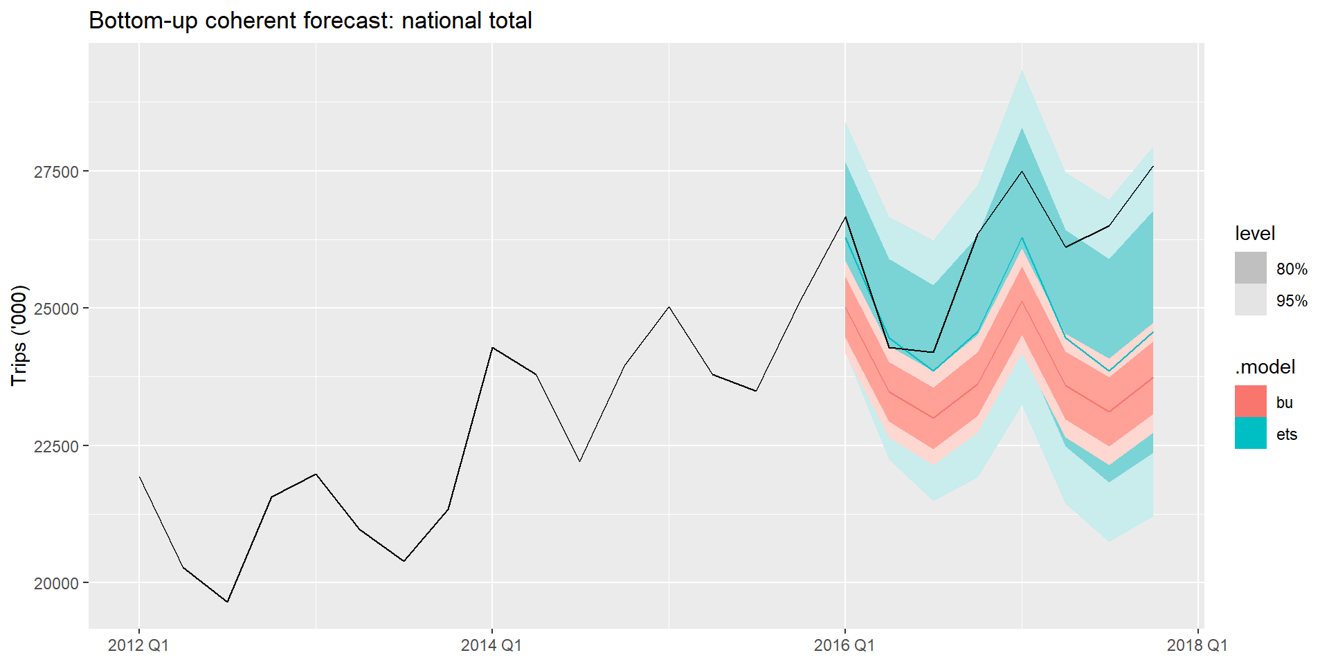
At the Region level, BU coherent forecasts are identical to the original ETS forecasts — nothing changes there.
| ✅ | Captures disaggregate dynamics. Best when bottom-level series have strong patterns. |
| ✅ | No need to forecast aggregate totals. |
| ❌ | Aggregate-level models are never used — wasteful if the total is well-behaved. |
| ❌ | Bottom-level series can be noisy; aggregating noisy forecasts amplifies errors. |
Forecast the top level (total), then disaggregate using historical proportions.
Three variants differ in how the proportions p_j are estimated:
Average historical proportions: p_j = \frac{1}{T}\sum_{t=1}^{T} \frac{y_{j,t}}{y_{\text{Total},t}} — time-average of per-period ratios.
Proportions of historical averages: p_j = \frac{\bar{y}_j}{\bar{y}_{\text{Total}}} — ratio of long-run averages. Less sensitive to periods with small totals than Method 1.
Forecast proportions: p_j computed from base forecasts at each level, not from history — adapts to structural changes.
reconcile()| ✅ | Aggregate model benefits from richer data. |
| ✅ | Simple to implement and explain to stakeholders. |
| ❌ | Historical proportions may not reflect future changes in mix. |
| ❌ | Bottom-level disaggregations lose any local dynamic not visible in the total. |
Choose a middle level as the anchor: aggregate upward (bottom-up logic), disaggregate downward (top-down logic).
tourism_mo <- tourism_fit |>
  reconcile(
1    mo = middle_out(ets, split = 1)
)split = 1 anchors on the level immediately below the total (State). State forecasts are taken as given; the national total aggregates up, and Region forecasts disaggregate down proportionally.
| ✅ | Middle level often has the richest signal: less noisy than the bottom, less aggregated than the top. |
| ✅ | Good compromise when the top-level series is hard to forecast. |
| ❌ | Choice of middle level is subjective and problem-dependent. |
| ❌ | Disaggregation below the middle level inherits the limitations of top-down proportions. |
| Method | Truth source | What changes? | Best when… |
|---|---|---|---|
| Bottom-Up | Bottom level | Top levels re-aggregated | Bottom series are informative and relatively clean |
| Top-Down | Top level | Bottom levels re-proportioned | Top-level dynamics dominate, bottom is too noisy |
| Middle-Out | Middle level | Top aggregated, bottom disaggregated | Middle level has the strongest signal |
All three methods treat one level as infallible and discard information from all others. No forecast level is truly noise-free — and that is exactly the gap that reconciliation methods fill.
tsibble.
Single-level approaches all share the same flaw: they assume one level’s forecasts are perfect and correct all others accordingly. In practice, every level has forecast errors.
MinT (Minimum Trace reconciliation) adjusts all levels simultaneously, using the statistical structure of forecast errors to find the best coherent set.
| Method | Who changes? |
|---|---|
| Bottom-Up | Top levels only |
| Top-Down / Middle-Out | Bottom levels only |
| MinT | Every level — including the bottom |
MinT borrows information across levels: a reliable national forecast pulls state forecasts toward proportional shares of the total. A well-forecasted state informs both the national aggregate and its sub-regions.
All reconciliation methods can be written as a linear transformation of the base forecasts:
\tilde{\mathbf{y}}_h = \mathbf{S}(\mathbf{S}'\mathbf{W}_h^{-1}\mathbf{S})^{-1}\mathbf{S}'\mathbf{W}_h^{-1}\hat{\mathbf{y}}_h
where:
The different min_trace() methods correspond to different estimators of \mathbf{W}_h.
For a three-series hierarchy (Total → A, B):
\mathbf{S} = \begin{pmatrix} 1 & 1 \\ 1 & 0 \\ 0 & 1 \end{pmatrix}
Row 1 (Total) = A + B. Row 2 (A) = A only. Row 3 (B) = B only. The solution \mathbf{P} = (\mathbf{S}'\mathbf{W}_h^{-1}\mathbf{S})^{-1}\mathbf{S}'\mathbf{W}_h^{-1} is the GLS estimator projected back through \mathbf{S}. Single-level approaches are special cases where \mathbf{W}_h assigns infinite weight to one level.
OLS minimizes squared errors treating all series equally — it ignores the fact that some series are more reliably forecast than others.
WLS assigns each series a weight inversely proportional to its forecast uncertainty. Series with smaller errors contribute more to the reconciled estimate. In the MinT framework, weights come from the diagonal of \mathbf{W}_h: higher variance → lower weight.
If the national total is much easier to forecast than any individual region, WLS pulls regional forecasts toward proportions of the reliable national forecast. OLS ignores this entirely.
min_trace()| Method | method = |
\mathbf{W}_h estimator | Notes |
|---|---|---|---|
| OLS | "ols" |
\mathbf{I} | Equal weights. Baseline. |
| WLS structural | "wls_struct" |
\text{diag}( series count ) | Weights from tree structure only — no data needed. |
| WLS variance | "wls_var" |
\text{diag}(\hat{\sigma}^2_j) | Weights from in-sample residual variances. |
| MinT sample | "mint_sample" |
Full sample covariance | Captures correlations. Unstable with many series. |
| MinT shrink | "mint_shrink" |
Regularized covariance | Recommended. Robust to limited data. |
"mint_shrink" applies a Ledoit-Wolf shrinkage estimator — regularizing toward a diagonal to avoid overfitting when the number of series is large relative to the number of observations.
tourism_rec <- tourism_fit |>
  reconcile(
    bu    = bottom_up(ets),
    td_ap = top_down(ets, method = "average_proportions"),
    td_pa = top_down(ets, method = "proportion_averages"),
    td_fp = top_down(ets, method = "forecast_proportions"),
    mo    = middle_out(ets, split = 1),
    wls   = min_trace(ets, method = "wls_struct"),
    mint  = min_trace(ets, method = "mint_shrink")
  )

tourism_fc <- tourism_rec |>
forecast(h = "2 years")tourism_fc |>
accuracy(data = tourism_hts, measures = list(RMSSE = RMSSE)) |>
mutate(
Level = case_when(
is_aggregated(State) ~ "Total",
!is_aggregated(State) & is_aggregated(Region) ~ "State",
TRUE ~ "Region"
)
) |>
group_by(.model, Level) |>
summarise(RMSSE = mean(RMSSE, na.rm = TRUE), .groups = "drop") |>
mutate(Level = factor(Level, levels = c("Total", "State", "Region")),
.model = fct_reorder(.model, RMSSE)) |>
ggplot(aes(x = .model, y = RMSSE, fill = .model)) +
geom_col(show.legend = FALSE) +
facet_wrap(~ Level, scales = "free_y") +
coord_flip() +
labs(x = NULL, y = "Mean RMSSE") +
theme_minimal()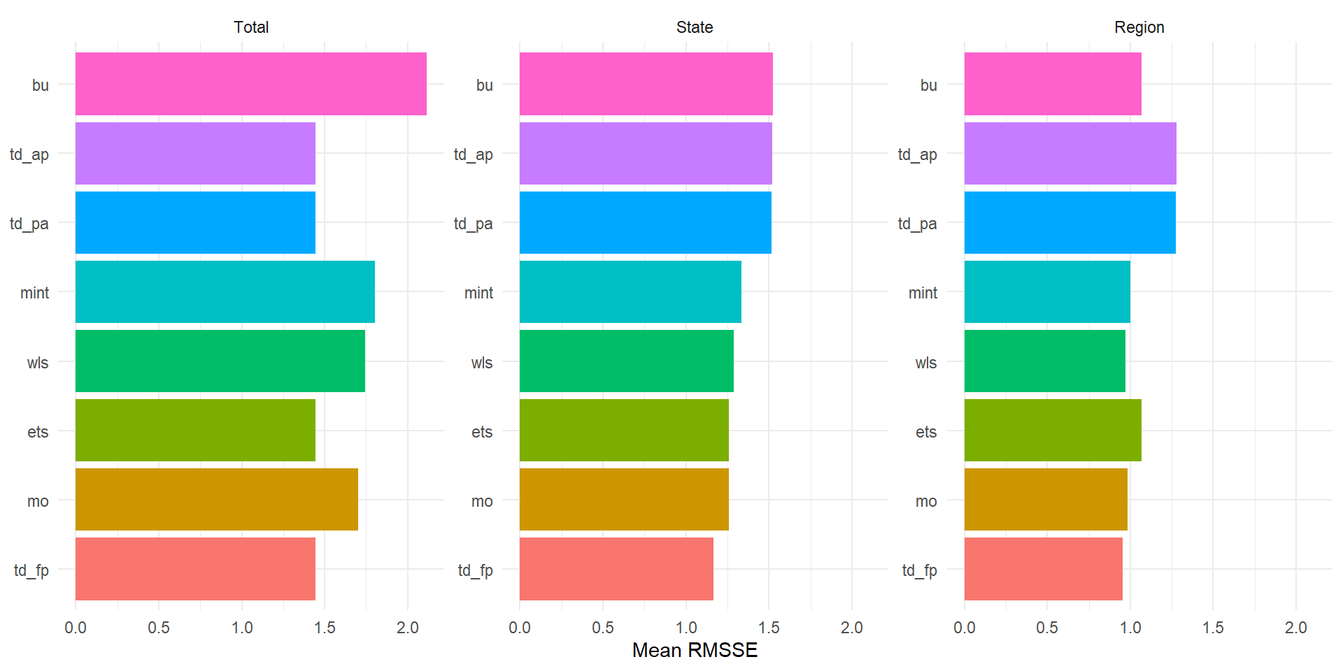
Single-level methods tend to perform best at their “home” level (BU at Region, TD at Total) and worse elsewhere. MinT shrink typically does well across all levels because it does not privilege any single level.
The PBS dataset records monthly Medicare Australia pharmaceutical prescriptions. It has a natural mixed structure: drug categories nest hierarchically (ATC1 → ATC2), and the Concession type (Concessional / General) is an independent grouping attribute.
ATC1 / ATC2 is the hierarchy; * Concession crosses it with the grouping attribute. Cost is scaled to millions.
pbs_fit <- pbs_train |>
  model(ets = ETS(Cost))

pbs_rec <- pbs_fit |>
  reconcile(
    bu   = bottom_up(ets),
    ols  = min_trace(ets, method = "ols"),
    wls  = min_trace(ets, method = "wls_struct")
  )

pbs_fc <- pbs_rec |>
forecast(h = "2 years")pbs_fc |>
accuracy(data = pbs_hts, measures = list(RMSSE = RMSSE)) |>
mutate(
Level = case_when(
is_aggregated(ATC1) ~ "Total",
!is_aggregated(ATC1) & is_aggregated(ATC2) & is_aggregated(Concession) ~ "ATC1",
!is_aggregated(ATC2) & is_aggregated(Concession) ~ "ATC2",
TRUE ~ "ATC2 × Concession"
)
) |>
group_by(.model, Level) |>
summarise(RMSSE = mean(RMSSE, na.rm = TRUE), .groups = "drop") |>
mutate(
Level = factor(Level, levels = c("Total", "ATC1", "ATC2", "ATC2 × Concession")),
.model = fct_reorder(.model, RMSSE)
) |>
ggplot(aes(x = .model, y = RMSSE, fill = .model)) +
geom_col(show.legend = FALSE) +
facet_wrap(~ Level, scales = "free_y") +
coord_flip() +
labs(x = NULL, y = "Mean RMSSE") +
theme_minimal()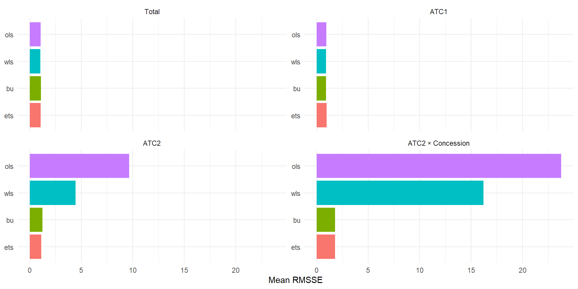
| Topic | Key takeaway |
|---|---|
| Structures | Hierarchical nests; grouped crosses; mixed combines both. |
aggregate_key() |
Defines the structure and computes all aggregations automatically. |
| Coherence | Forecasts that don’t add up create operational inconsistencies. |
| Bottom-Up | Safe default when bottom-level series are informative. |
| Top-Down | Three variants; forecast proportions is usually preferable. |
| Middle-Out | Useful when the middle level has the strongest signal. |
| MinT | Adjusts all levels jointly. mint_shrink is the recommended default. |
bottom_up() as your baseline.min_trace(method = "mint_shrink") alongside it.accuracy() faceted by aggregation level.