Stationarity & Differencing

Modified

March 29, 2026

Code

1library(tidyquant)
library(plotly)

1: In addition to the regular packages, here we’ll use tidyquant and plotly.

1 Stationarity

Have you ever heard the word “stationary” before?

Gas cylinders & stationary tanks — what’s the difference?

In everyday language, stationary means not moving — fixed in place.
For a time series, what would that mean?

Think about it

If a time series is “not moving”, what statistical properties would you expect it to have?

1.1 The Formal Definition

A time series is stationary if its statistical properties — primarily its mean and variance — do not change over time.

The series fluctuates around a constant mean.
The spread of those fluctuations stays roughly constant over time.
There are no systematic patterns that change the level or scale of the series.

1.2 Are These Series Stationary?

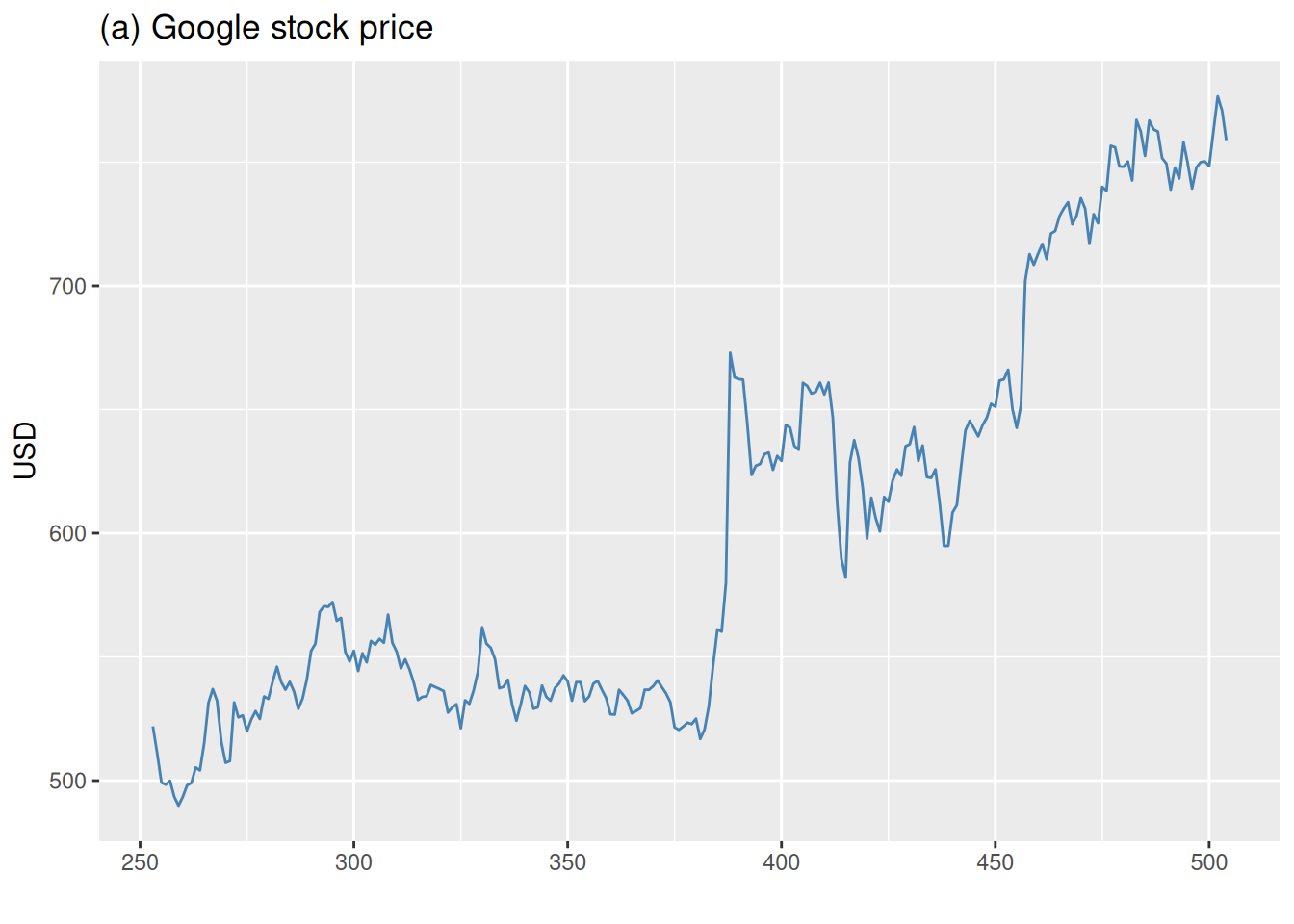
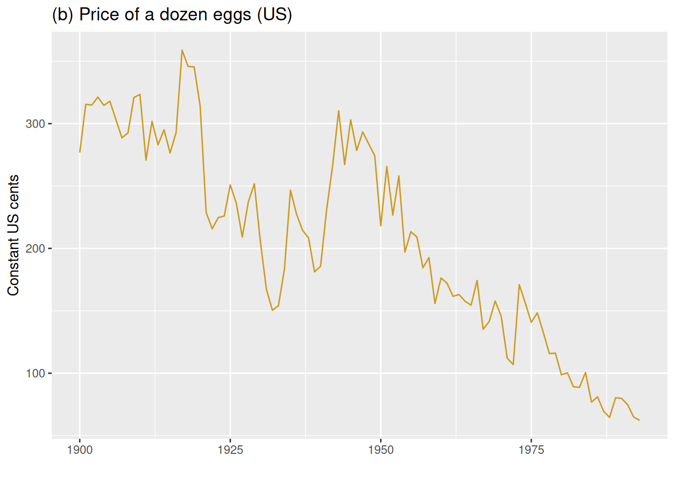
Which of the following six series are stationary (i.e., which look more stable)?

Answer

(a) and (b): clear trends (upward and downward) → not stationary ✗
(c) and (d): strong repeating seasonal pattern → not stationary ✗
(e): daily returns fluctuate around zero with constant spread → stationary ✓
(f): the cycling looks seasonal but has no fixed period — this is a business cycle. The series is stationary ✓

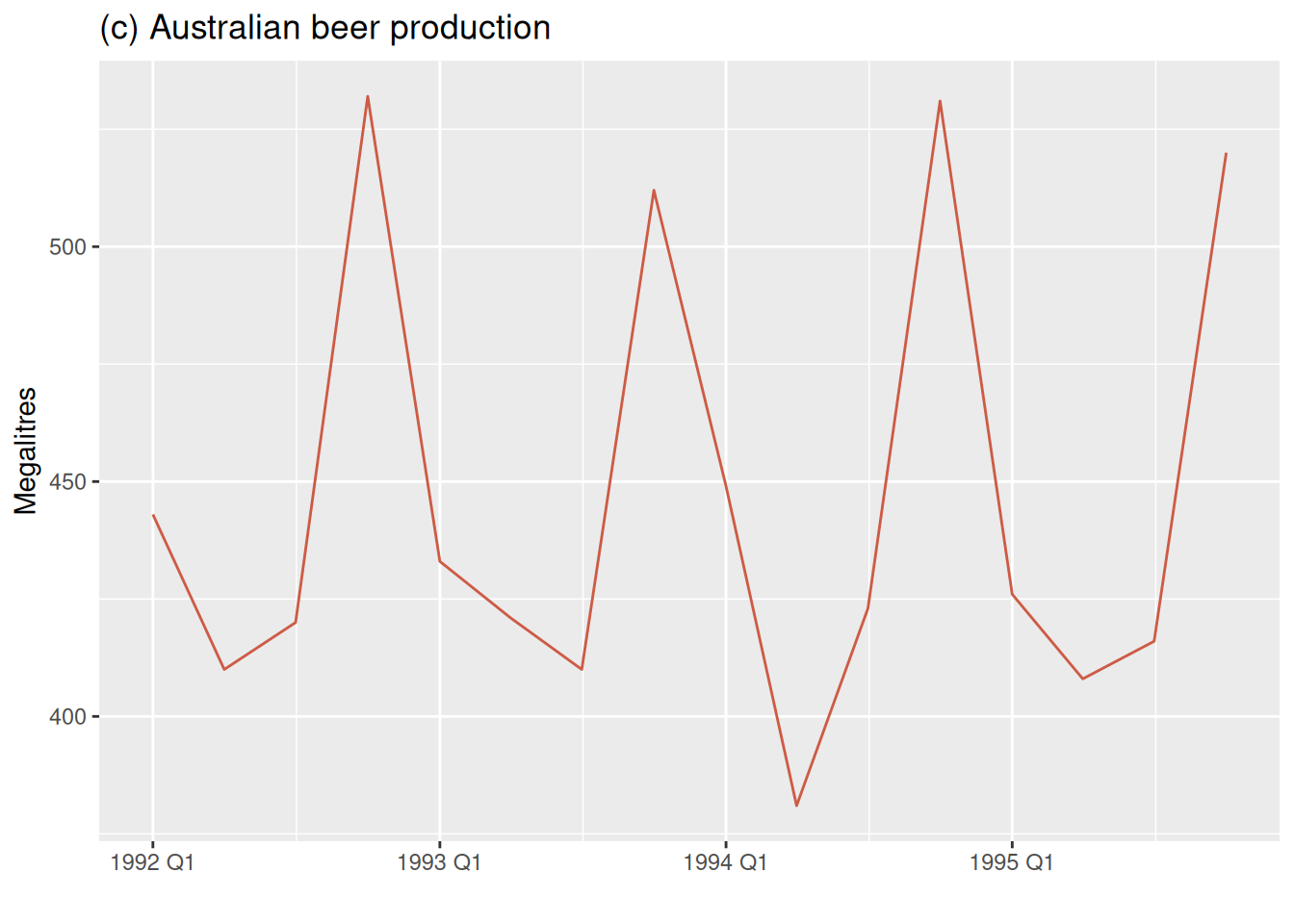
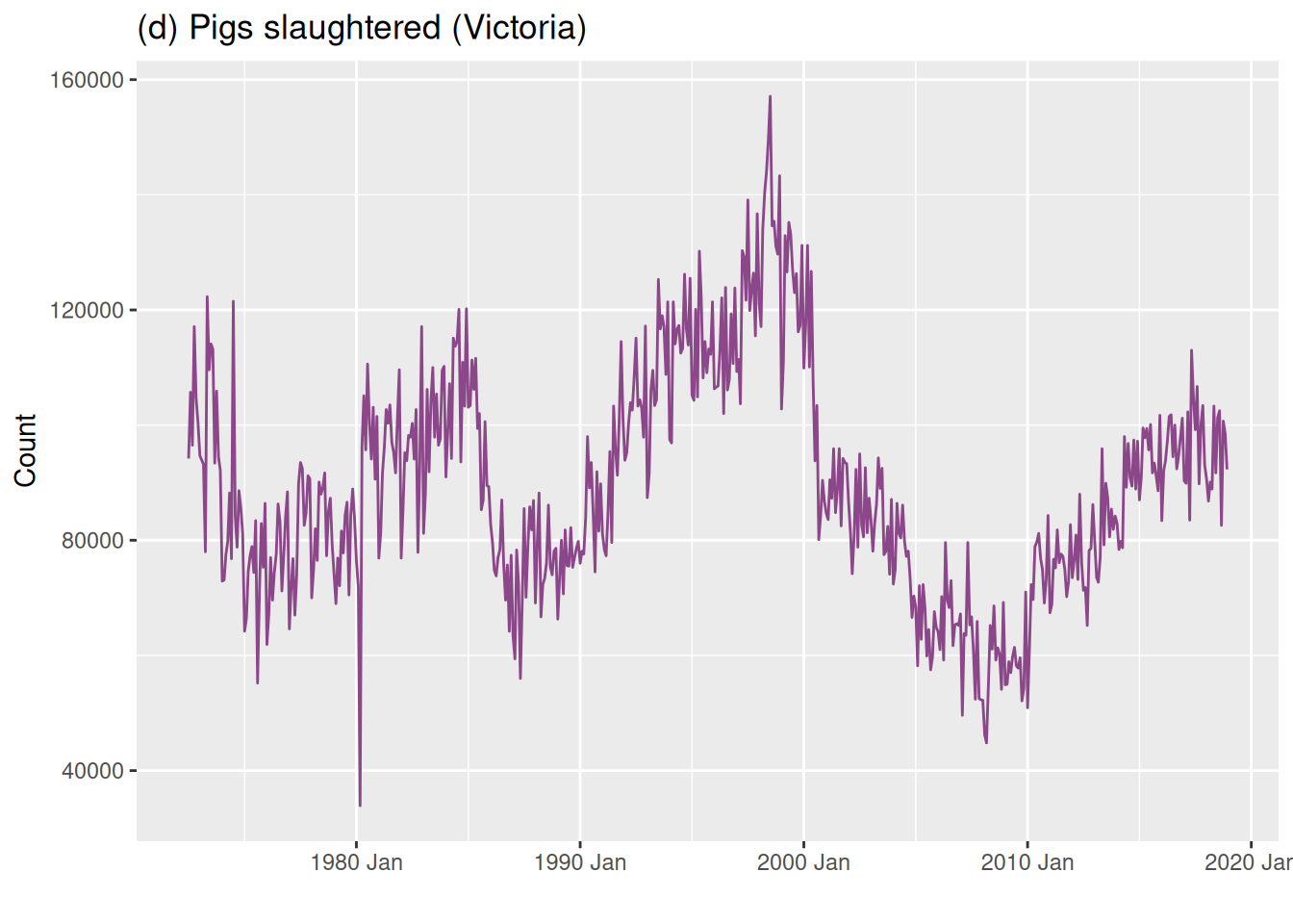
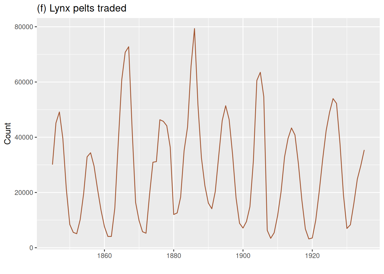
Key distinction: Seasonality repeats at a fixed, known frequency. Business cycles rise and fall irregularly.

1.3 What Makes a Series Non-Stationary?

A time series is non-stationary if it exhibits any of the following:

Trend — a long-term increase or decrease in the mean.
Seasonality — a repeating pattern that causes the mean to shift systematically.
Changing variance — the spread of fluctuations grows or shrinks over time.

What can we expect from a Stationary Series then?

A stationary serie will not have any systematic patterns that change the level or scale of the series over time (no trend, no seasonality, and constant variance).

1.4 Why Does Stationarity Matter?

There is an important family of forecasting models that work by describing the correlation structure between a series and its own past values.
For those correlations to be stable and meaningful, the series needs to be stationary.

The key question

If these models require stationarity, does that mean they can only work with series that have no trend, no seasonality, and no changing variance?
Or is there something we can do to a non-stationary series to make it usable?

1.5 What to do with Non-Stationary Series?

1.5.1 If we find heteroskedasticity (changing variance)

Recall from Module 1: we can stabilize the variance using mathematical transformations — logarithms, Box-Cox, and so on.

1.5.2 But what about the mean?

Transformations alone don’t remove a trend or seasonal pattern.

2 Differencing

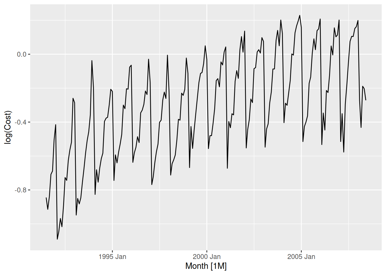
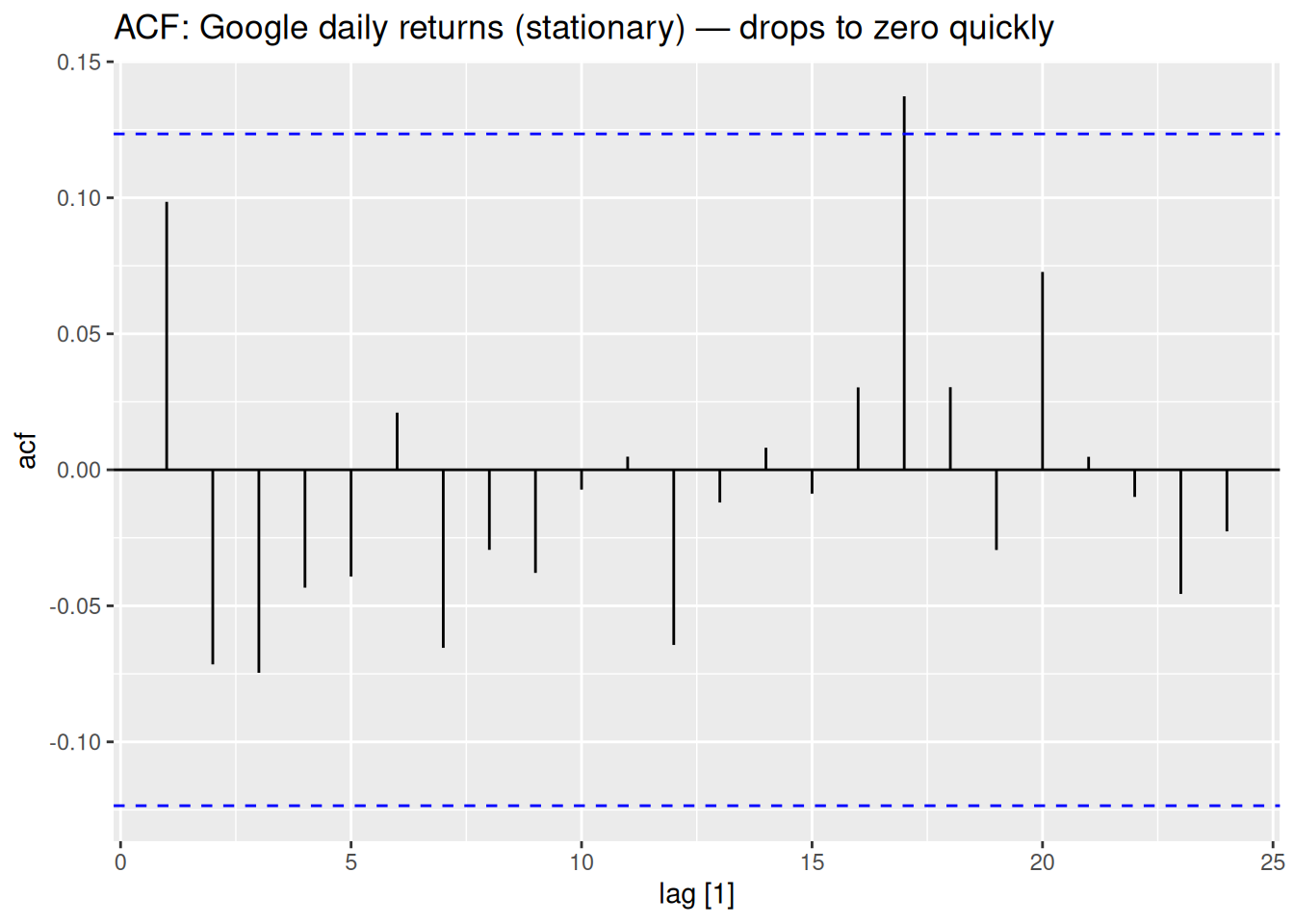
Look at these two series:

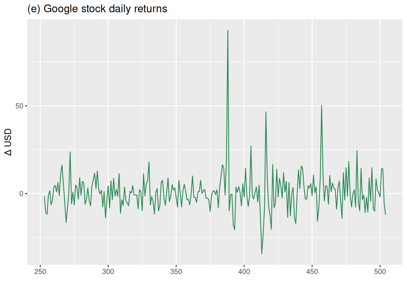
The second series was produced directly from the first. Can you figure out how?

Differencing

The daily return is simply today’s price minus yesterday’s price — the change between consecutive observations. This operation is called differencing, and it is how we stabilize the mean of a non-stationary series.

Random walks & stationarity

Google’s stock price follows a random walk.
By definition, random walks are non-stationary, but their first differences are stationary.

2.1 First Differences

The first difference of a series y_t is:

y'_t = y_t - y_{t-1}

The differenced series has T - 1 observations.
First differences represent the change from one period to the next.
If the original series has a linear trend, the differences will fluctuate around a constant mean.

Code

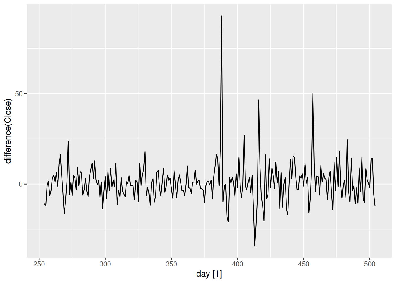
google_2015 |>
1  autoplot(difference(Close))

1: difference(Close) computes the first difference of the Close variable.

2.2 Second Differences

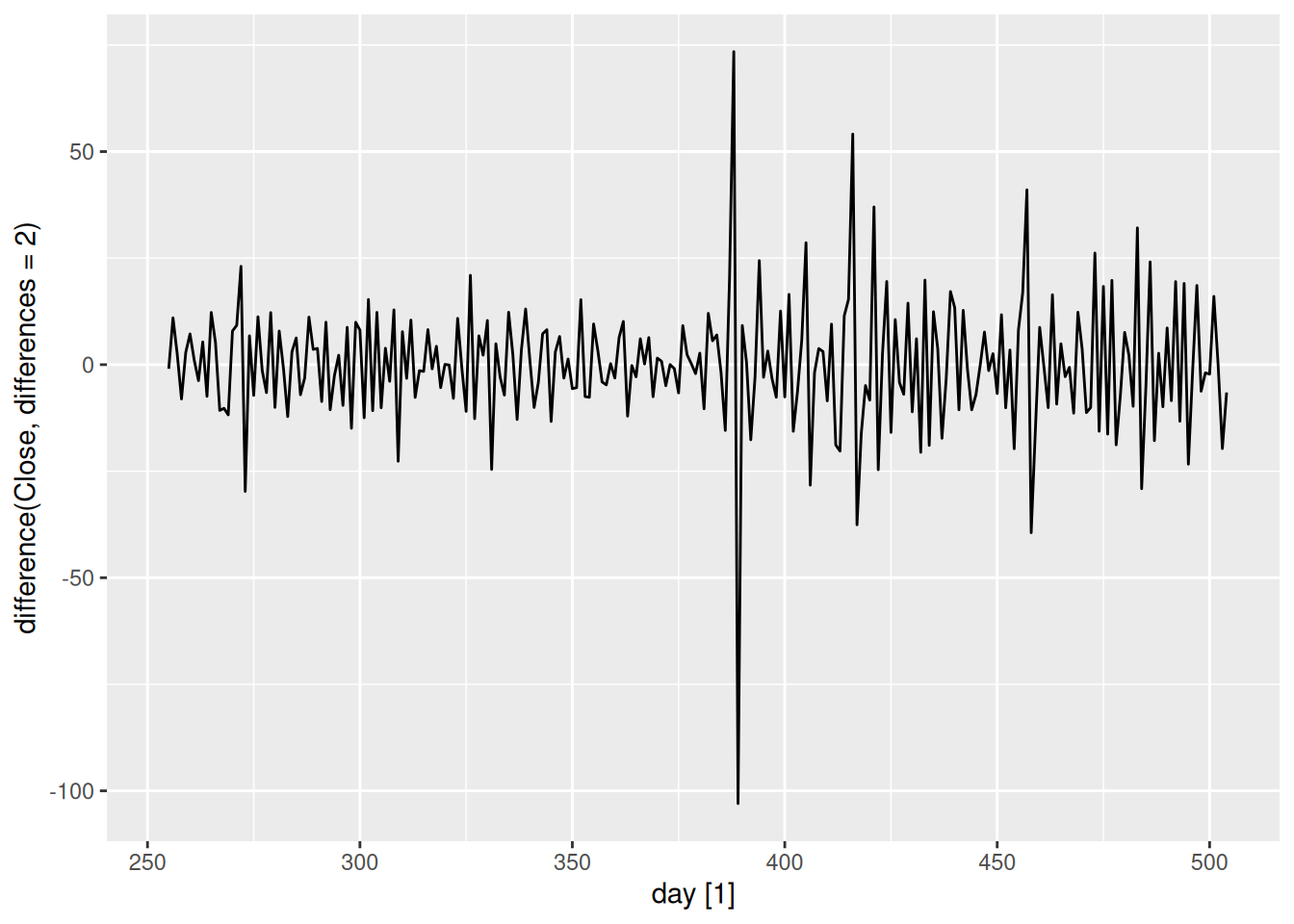
Sometimes the first-differenced series is still non-stationary. We can difference again:

\begin{align*} y''_t &= y'_t - y'_{t-1} \\ &= (y_t-y_{t-1}) - (y_{t-1} - y_{t-2}) \\ &= y_t - 2y_{t-1} + y_{t-2} \end{align*}

Second differences have T - 2 observations.
They represent the change in the changes — acceleration rather than velocity.
Economic and business series almost never require more than two differences.

Needing three or more differences usually signals something else is wrong — an outlier, a structural break, or a transformation that should have been applied first.

Code

google_2015 |>
1  autoplot(difference(Close, differences = 2))

1: The argument differences = 2 tells difference() to apply the differencing operation twice.

2.3 Seasonal Differencing

If the series has seasonality, we take a seasonal difference — the change relative to the same period in the previous cycle:

y'_t = y_t - y_{t-m}

where m is the seasonal period (m = 12 for monthly data, m = 4 for quarterly, …).

Seasonal differences represent season-over-season change¹ at each point.
Also called lag-m differences.
After seasonal differencing, any remaining non-seasonal trend can be removed with a first difference.

Code

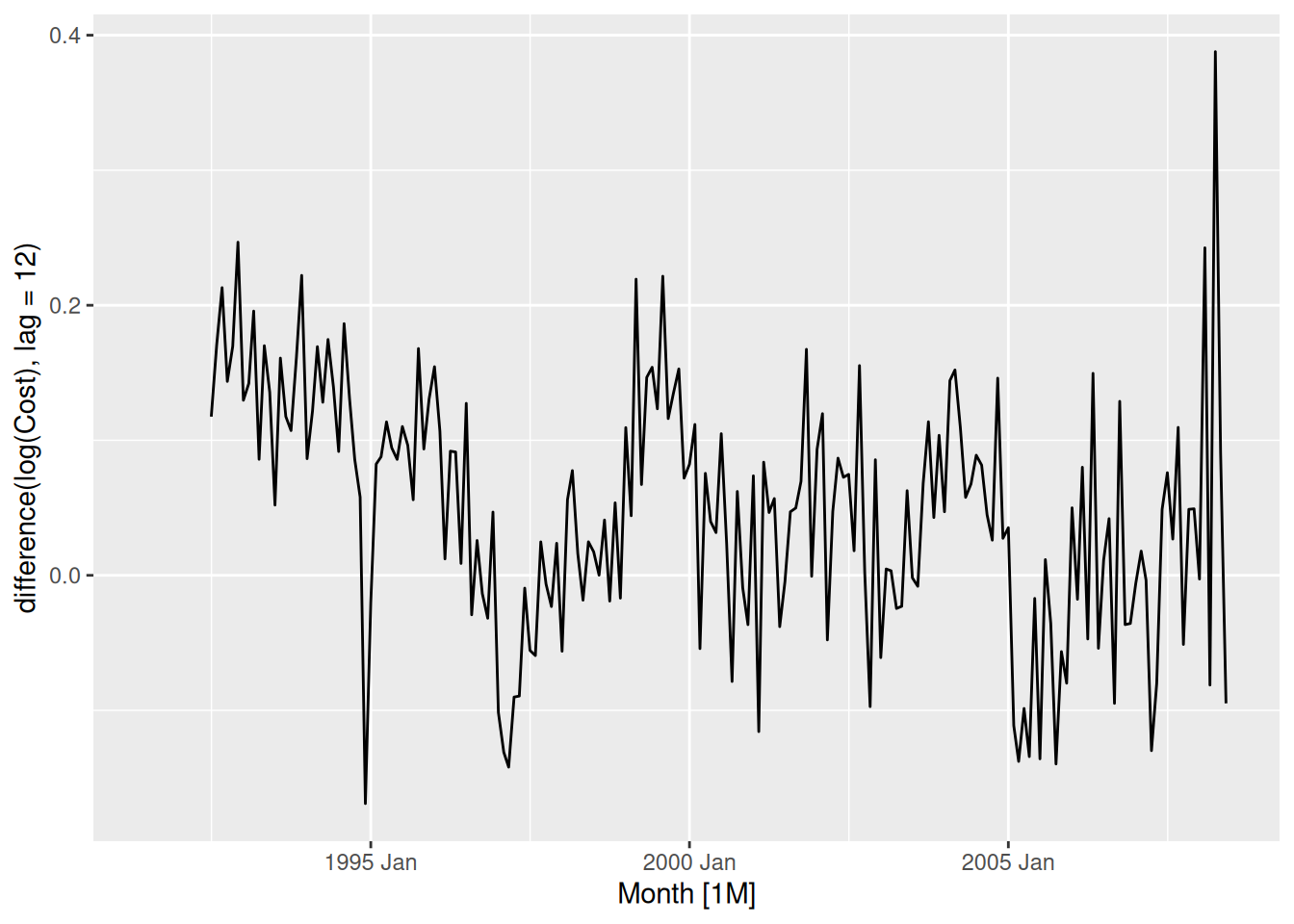
h02 |>
1  autoplot(difference(log(Cost), lag = 12))

1: The argument lag = 12 tells difference() to compute the seasonal difference with a lag of 12 periods (i.e. y_t - y_{t-12}). If no lag is specified, it defaults to 1 (the first difference).

2.4 Does the Order of Differencing Matter?

When a series needs both seasonal and regular differencing, does it matter which one we apply first?

Applying seasonal first, then regular:

\begin{align*} (y_t - y_{t-m})' &= (y_t - y_{t-m}) - (y_{t-1} - y_{t-m-1}) \\ &= y_t - y_{t-1} - y_{t-m} + y_{t-m-1} \end{align*}

Applying regular first, then seasonal:

\begin{align*} (y_t - y_{t-1})' &= (y_t - y_{t-1}) - (y_{t-m} - y_{t-m-1}) \\ &= y_t - y_{t-1} - y_{t-m} + y_{t-m-1} \end{align*}

Both routes lead to the same result.

The order does not matter — the result is always identical. In practice, if the seasonal pattern is strong, apply the seasonal difference first: the result may already be stationary without needing the regular difference.

2.5 Backshift Notation

The backshift operator B provides a compact way to write differencing operations — and, as we will see next class, to write out full model equations cleanly.

It is defined simply as:

By_t = y_{t-1} ; B(By_t) = B^2 y_t = y_{t-2}

That is, applying B to a series shifts it back one period.

2.5.1 First Differences

Recall the first difference:

y'_t = y_t - y_{t-1}

We can rewrite y_{t-1} = By_t, so:

y'_t = y_t - By_t = (1 - B)y_t

2.5.2 Second Differences

Recall:

y''_t = y_t - 2y_{t-1} + y_{t-2}

Using the backshift operator turns to:

y''_t = y_t - 2By_t + B^2 y_t = (1 - 2B + B^2)y_t

which gives a perfect square trinomial²

y''_t = (1-B)^2 y_t

2.5.3 General d-level Differences

The pattern generalizes naturally:

(1 - B)^d y_t

where d is the number of times we difference the series.

Binomial expansion of (1-B)^d

For a general order d, the binomial theorem gives:

(1-B)^d = \sum_{k=0}^{d} \binom{d}{k} (-B)^k = \sum_{k=0}^{d} \binom{d}{k} (-1)^k B^k

So:

(1-B)^d y_t = \sum_{k=0}^{d} \binom{d}{k} (-1)^k y_{t-k}

For d=1: y_t - y_{t-1} ✓
For d=2: y_t - 2y_{t-1} + y_{t-2} ✓

2.5.4 Seasonal Differences

A seasonal difference shifts back m periods:

y_t - y_{t-m} = y_t - B^m y_t = (1 - B^m)y_t

And when both are needed — as with mexretail — the two operators simply multiply:

(1-B)(1-B^m)y_t

which is exactly the expression we expanded by hand in the previous section.

Operation	Backshift form
First difference	(1 - B)\,y_t
Second difference	(1 - B)^2\,y_t
d-th difference	(1 - B)^d\,y_t
Seasonal difference	(1 - B^m)\,y_t
Both together	(1 - B)^d(1 - B^m)\,y_t

Order of differencing — revisited

Using backshift notation, it becomes trivial to see that the order doesn’t matter. Both orderings produce the same expression, since multiplication is commutative:

(1-B)(1-B^m)y_t = (1-B^m)(1-B)y_t

No algebra needed.

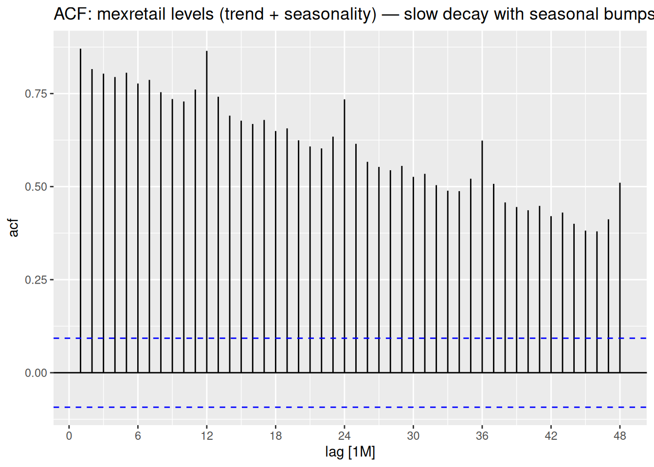
2.6 Applying This to `mexretail`

mexretail has trend, seasonality, and growing variance. The full differencing pipeline:

We have been deciding how many differences to apply by looking at plots. But visual inspection is subjective — two analysts could disagree. Is there a more rigorous, objective way to make this call?

3 Unit Root Tests

Visual inspection is useful but subjective. Unit root tests formalize the question: is this series stationary?

The test we will use is the KPSS test (Kwiatkowski-Phillips-Schmidt-Shin).

The KPSS statistic

The KPSS test works by regressing y_t on a constant (or a constant + trend), computing the residuals e_t, and then building their cumulative sums S_t = \sum_{i=1}^{t} e_i. The test statistic is:

\text{KPSS} = \frac{1}{T^2} \sum_{t=1}^{T} \frac{S_t^2}{\hat{\sigma}^2}

where \hat{\sigma}^2 is a long-run variance estimate that corrects for autocorrelation in the residuals.

The intuition: if the series is stationary, the residuals e_t fluctuate around zero and their cumulative sums S_t stay bounded. If the series has a unit root (non-stationary), the cumulative sums drift away from zero — making the statistic large and leading to rejection of H_0.

Read the hypotheses carefully — they are the opposite of what you might expect

H_0: \text{the series IS stationary} H_1: \text{the series is NOT stationary}

Large p-value (> 0.05): fail to reject H_0 → the series is stationary ✓
Small p-value (< 0.05): reject H_0 → the series needs differencing ✗

You want a large p-value here.

3.1 KPSS in R

Code

google_2015 |> features(Close, unitroot_kpss)

Code

google_2015 |> features(diff_close, unitroot_kpss)

3.2 Automated Differencing Orders

Rather than manually testing each transformation, feasts provides two functions that determine exactly how many differences are needed:

Code

mexretail |> features(box_cox(y, lambda), unitroot_nsdiffs)

Code

mexretail |>
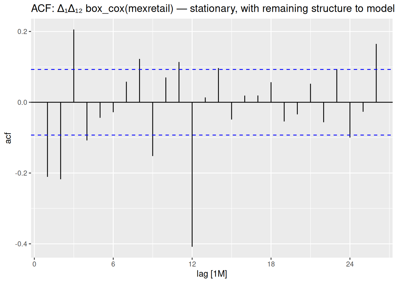
  features(difference(box_cox(y, lambda), 12), unitroot_ndiffs)

Full stationarity protocol for mexretail

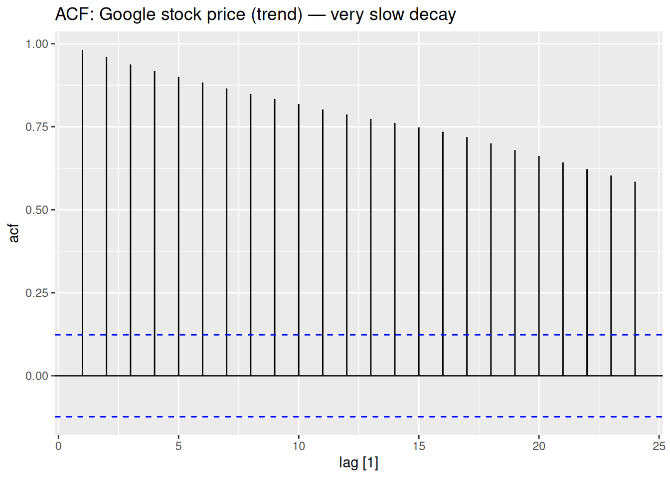
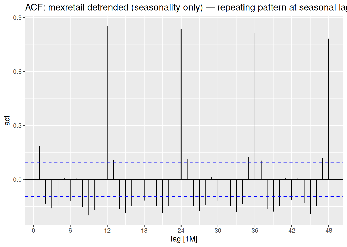
Apply Box-Cox with Guerrero lambda to stabilize variance: box_cox(y, lambda)
Check seasonal differencing needed: unitroot_nsdiffs() → 1
Apply seasonal diff, then check regular: unitroot_ndiffs() → 1
Final stationary series: difference(box_cox(y, lambda), 12) |> difference(1)

4 ACF and PACF

We have already encountered the ACF when diagnosing residuals from our benchmark models — checking whether leftover errors looked like white noise. Here we use it for a different but related purpose: understanding the correlation structure of the series itself.

4.1 Autocorrelation Function (ACF)

The ACF measures the correlation between a series and its own past values at each lag k:

r_k = \text{Corr}(y_t,\, y_{t-k})

ACF as a stationarity diagnostic

Stationary series: ACF drops to zero quickly.
Non-stationary series: ACF decays very slowly, with the lag-1 value close to 1.

This gives us another way to detect non-stationarity — and, as we will see, it also tells us about the structure of the model to fit.

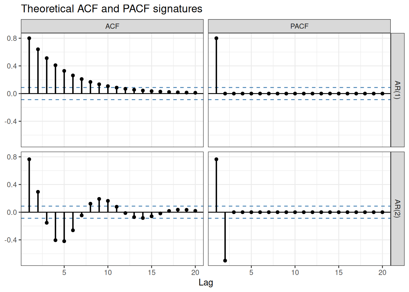
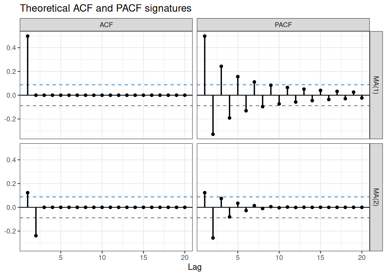
4.2 ACF Shapes for Different Patterns

4.3 Partial Autocorrelation Function (PACF)

The ACF at lag k captures both the direct relationship between y_t and y_{t-k} and the indirect relationship mediated through intermediate lags. The PACF isolates only the direct part.

The regression analogy

ACF at lag k: simple correlation between y_t and y_{t-k}.
PACF at lag k: the coefficient on y_{t-k} in a regression of y_t on y_{t-1}, y_{t-2}, \ldots, y_{t-k}.

The PACF asks: once I already know the effect of all closer lags, does lag k add any new information?

4.4 ACF and PACF Together

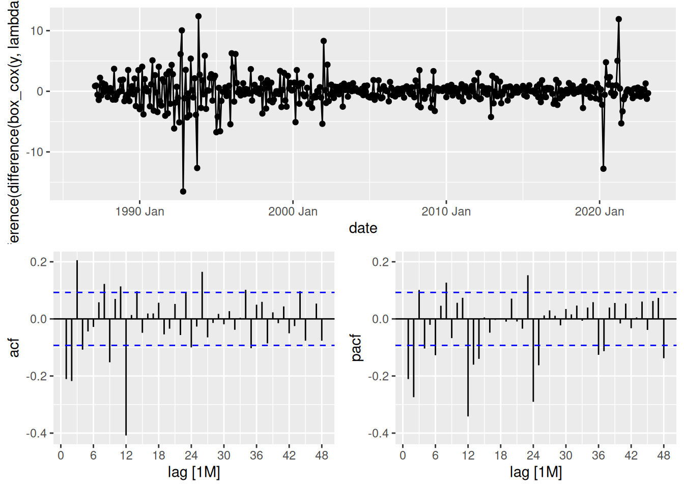
gg_tsdisplay() with plot_type = "partial" shows the time series, ACF, and PACF together — this is the standard diagnostic display for the rest of the module.

Code

mexretail |>
  gg_tsdisplay(
    difference(box_cox(y, lambda), 12) |> difference(1),
    plot_type = "partial",
    lag_max = 48
  )

5 AR and MA Models

5.1 Autoregressive Models — AR(p)

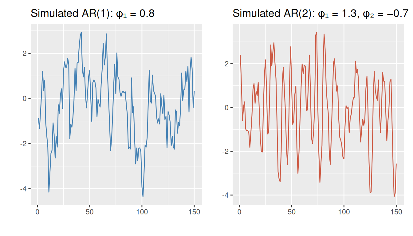
An autoregressive model of order p forecasts y_t as a weighted sum of its own past values:

y_t = c + \phi_1 y_{t-1} + \phi_2 y_{t-2} + \cdots + \phi_p y_{t-p} + \varepsilon_t

Structurally identical to multiple linear regression — except the predictors are lagged values of the series itself.
p is the number of past values used.
\varepsilon_t is white noise.

Signature in ACF/PACF

PACF cuts off sharply after lag p — this is how you read the order.
ACF decays exponentially or sinusoidal.

5.2 Moving Average Models — MA(q)

A moving average model of order q forecasts y_t as a weighted sum of past forecast errors:

y_t = c + \varepsilon_t + \theta_1 \varepsilon_{t-1} + \theta_2 \varepsilon_{t-2} + \cdots + \theta_q \varepsilon_{t-q}

The predictors are past errors, not past values of the series.
q is the number of past errors used.
\varepsilon_t is white noise.

MA models ≠ moving average smoothing

Do not confuse MA models with the moving average smoothing used in decomposition. Smoothing estimates the trend-cycle from past observed values. MA models use past errors to describe the correlation structure of the series.

Signature in ACF/PACF

ACF cuts off sharply after lag q — the mirror image of the AR signature.
PACF decays exponentially or sinusoidal.

You cannot identify a model from the time plot alone

Now that you have seen AR and MA models: their time plots can look very similar to each other. The ACF and PACF are what distinguish them. This is fundamentally different from ETS, where the form of trend and seasonality in the time plot directly guides model selection — one of the key differences we will revisit when comparing these two families.

5.3 What Comes Next

In practice, you will rarely use a pure AR or pure MA model. Real series typically need both. And most real series also need differencing before any of this applies.

Combining differencing, AR terms, and MA terms into a single unified model — and applying it systematically to mexretail — is the subject of the next class.

Where we are in the bigger picture

Stabilize variance → Box-Cox / log transformation ✓
Stabilize the mean → differencing ✓
Detect remaining correlation structure → ACF and PACF ✓
Understand the building blocks → AR and MA terms ✓

All the pieces are in place. Time to put them together.

Footnotes

most commonly YoY (year-over-year), but remember there can be daily, weekly, or more seasonal patterns too.↩︎
↩︎

1 Stationarity

1.1 The Formal Definition

1.2 Are These Series Stationary?

1.3 What Makes a Series Non-Stationary?

1.4 Why Does Stationarity Matter?

1.5 What to do with Non-Stationary Series?

1.5.1 If we find heteroskedasticity (changing variance)

1.5.2 But what about the mean?

2 Differencing

2.1 First Differences

2.2 Second Differences

2.3 Seasonal Differencing

2.4 Does the Order of Differencing Matter?

2.5 Backshift Notation

2.5.1 First Differences

2.5.2 Second Differences

2.5.3 General d-level Differences

2.5.4 Seasonal Differences

2.6 Applying This to mexretail

3 Unit Root Tests

3.1 KPSS in R

3.2 Automated Differencing Orders

4 ACF and PACF

4.1 Autocorrelation Function (ACF)

4.2 ACF Shapes for Different Patterns

4.3 Partial Autocorrelation Function (PACF)

4.4 ACF and PACF Together

5 AR and MA Models

5.1 Autoregressive Models — AR(p)

5.2 Moving Average Models — MA(q)

5.3 What Comes Next

Footnotes

2.6 Applying This to `mexretail`