- 1
- For interactive plots.
- 2
-
For the
vif()function used in the multicollinearity section.
Linear Regression Models for Time Series
1 From Univariate to Multivariate Models
Every model we have built so far shares one fundamental characteristic: it is univariate. Whether it was STL decomposition, ETS, or ARIMA, we only looked inward — we used the history of y_t itself to forecast its future.
That approach has taken us surprisingly far. But it ignores the outside world entirely.
- A retailer’s sales are not just a function of past sales — they depend on promotions, competitor prices, and economic conditions.
- Energy demand depends on temperature, not just its own history.
- Mexico’s retail trade index (
mexretail) reflects consumer purchasing power, employment, and credit conditions — none of which appear in the series itself.
1.1 Why exogenous variables?
The question we are addressing now is: what if we gave our model access to external information?
- In Modules 1–2, our model improved by getting smarter about the structure of y_t (trend, seasonality, autocorrelation).
- In Module 3, we improve by adding context: variables from outside the series that help explain its movement.
- This is the transition from filtering to causal modeling — at least in the predictive, not necessarily structural, sense.
NoteWhere we’ve been and where we’re going
| Module | What we modeled | Tool |
|---|---|---|
| 1 | Trend + seasonality via decomposition | STL + SNAIVE/Drift |
| 2 | Autocorrelation structure of the signal | ETS, ARIMA |
| 3 | Relationship with external variables | TSLM, dynamic regression |
| 4 | Complex seasonality, robustness | Prophet, bootstrapping |
Each module has asked: what does my current model fail to capture? The answer now is: information from other series.
2 The Linear Regression Model
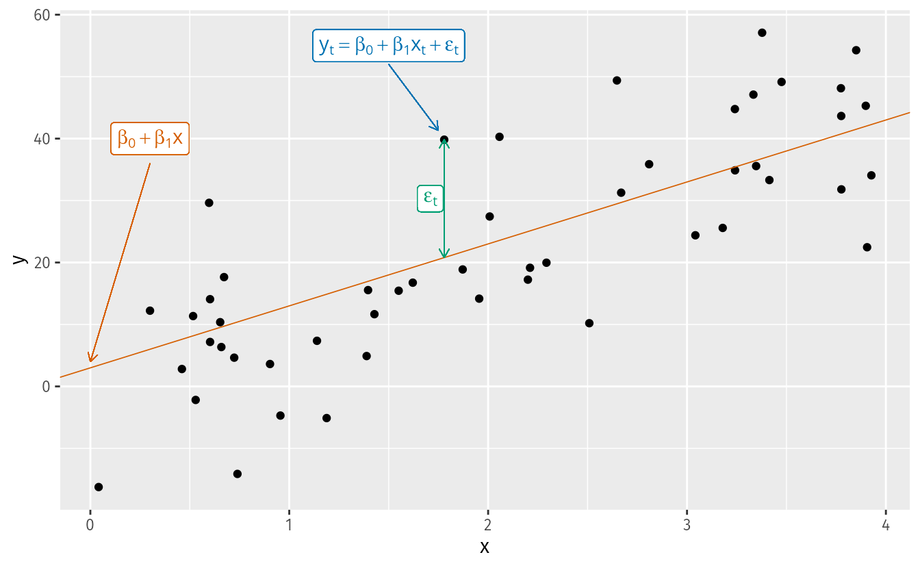
The simplest case is the simple linear regression model:
y_t = \beta_0 + \beta_1 x_t + \varepsilon_t
where:
- \beta_0 is the intercept: the predicted value of y when x = 0.
- \beta_1 is the slope: the average change in y for a one-unit change in x.
- \varepsilon_t is the error term: captures all other influences on y_t not explicitly modeled.
TipHow are the \beta’s estimated? Ordinary Least Squares (OLS)
We cannot observe the \beta’s directly — we estimate them from data. The Ordinary Least Squares (OLS) method chooses the estimates \hat{\beta}_0, \hat{\beta}_1, \ldots, \hat{\beta}_k that minimize the sum of squared residuals:
\min_{\hat{\boldsymbol{\beta}}} \sum_{t=1}^{T} \hat{\varepsilon}_t^2 = \sum_{t=1}^{T} \left(y_t - \hat{\beta}_0 - \hat{\beta}_1 x_{1t} - \cdots - \hat{\beta}_k x_{kt}\right)^2
For the simple case (k = 1), taking partial derivatives and setting them to zero yields closed-form solutions:
\hat{\beta}_1 = \frac{\sum x_t y_t - T\bar{x}\bar{y}}{\sum x_t^2 - T\bar{x}^2}, \qquad \hat{\beta}_0 = \bar{y} - \hat{\beta}_1 \bar{x}
For the general case with k predictors, the solution extends naturally to matrix form:
\hat{\boldsymbol{\beta}} = (\mathbf{X}^\top \mathbf{X})^{-1} \mathbf{X}^\top \mathbf{y}
where \mathbf{X} is the design matrix — a column of ones (for the intercept) plus one column per predictor — and \mathbf{y} is the vector of observed responses.
In practice, R handles all of this internally. But knowing the objective function matters: OLS penalizes large residuals more than small ones (because of the square), and under the classical assumptions the Gauss-Markov theorem guarantees the estimates are BLUE (Best Linear Unbiased Estimators) — regardless of whether we have one predictor or twenty.
2.1 Some motivating examples
- Ice cream sales (y) and daily temperature (x).
- Nike revenue (y) and marketing spend (x).
- US consumption growth (y) and income growth (x).
- Mexico retail trade (y) and consumer confidence index (x).
NoteTerminology: many names for y and x
The same concept appears under different names depending on the discipline:
| y (forecast variable) | x (predictor variables) |
|---|---|
| Dependent | Independent |
| Explained | Explanatory |
| Regressand | Regressor |
| Response | Stimulus / Covariate |
| Endogenous | Exogenous |
In time series forecasting, FPP3 uses forecast variable and predictor variables.
NoteThe origin of “regression” — Galton, 1886
The term was coined by Francis Galton while studying the relationship between parents’ height and their children’s height.
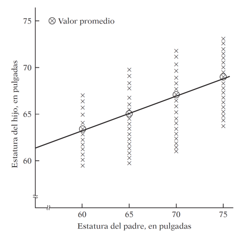
His finding: tall parents tend to have tall children, but on average their children are not as tall as them. Short parents tend to have children taller than themselves. There is a tendency to regress toward the mean.
Without this regression to the mean, the distribution of heights across generations would diverge — we would eventually have people of Hobbit stature and people of giant stature, with nothing in between.
Modern regression analysis generalizes this idea: studying the dependence of one variable on one or more others to predict its average value.
2.2 Regression and Causality
“A statistical relationship, however strong and suggestive, can never establish causal connexion: our ideas of causality must come from outside statistics, ultimately from some theory or other.”
— Kendall & Stuart (1961)
\text{Regression} \neq \text{Causality} \qquad \text{Correlation} \neq \text{Causality}
This is not a technicality — it is one of the most practically important ideas in data science:
- People who carry lighters have higher rates of lung cancer. Does carrying a lighter cause cancer?
- Ice cream sales and drowning rates are correlated. Should we ban ice cream?
- Homeopathic treatments show improvements. Does the remedy work, or did patients improve on their own?
- Casually: “every time I hiccup and hold my breath, it goes away.” Does holding your breath cure hiccups, or would they have stopped anyway?
2.2.1 Spurious correlations
The web is full of striking examples where two completely unrelated time series happen to move together — these are called spurious correlations.
Important
A regression model would happily fit a line through any of those charts. The model does not know the relationship is nonsense — you have to know. Causal direction requires theory, domain knowledge, or experimental design, not statistical strength alone.
2.3 What Does “Linear” Mean?
Are these models linear?
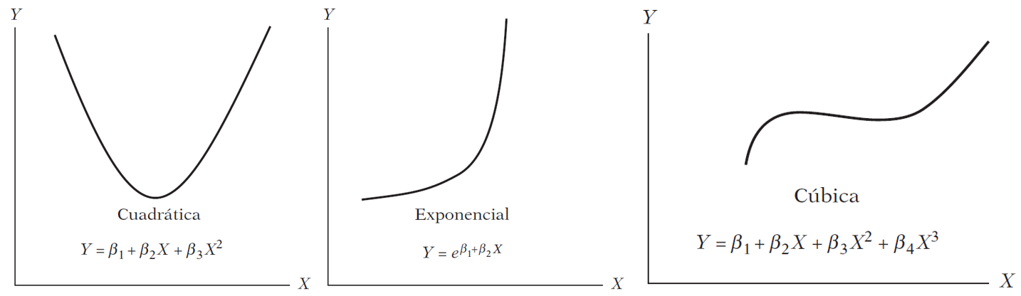
Linearity can be defined in two senses:
Linearity in the variables — E(y \mid x) is a linear function of x. This is the restrictive sense: only straight lines.
Linearity in the parameters — E(y \mid x) is linear in the \beta’s.
The three models above are all nonlinear in x but linear in \beta. A linear regression model can produce a straight line, a parabola, an exponential curve, or a piecewise function, depending on the functional form chosen.
3 Regression in R: us_change
We will use us_change — quarterly percentage changes in US macroeconomic variables. Our forecast variable is Consumption.
Code
us_change3.1 Exploratory analysis
Before fitting any model, we look at the data.
Code
us_change |>
  as_tibble() |>
  select(-Quarter) |>
  GGally::ggpairs()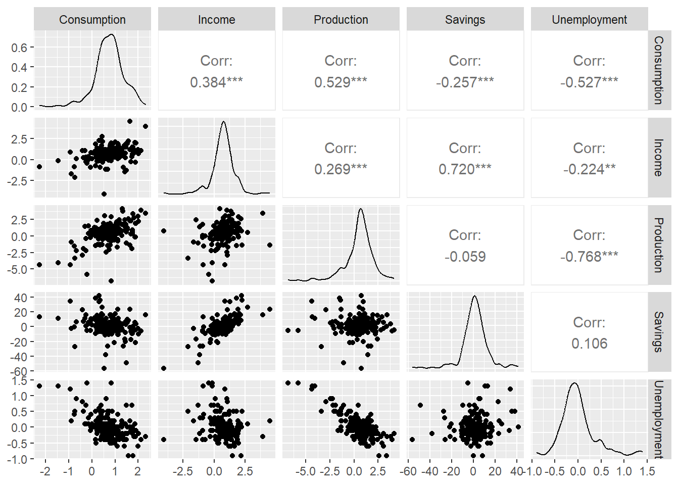
The scatter matrix shows correlations between all pairs of variables. Notice that some predictors are correlated with each other — we will return to this when we discuss multicollinearity.
3.2 Simple Linear Regression
We start with the simplest possible model: Consumption as a function of Income only.
y_{t, \text{Consumption}} = \beta_0 + \beta_1 x_{t, \text{Income}} + \varepsilon_t
In fable, time series linear models use TSLM():
Code
- 1
-
Start with the
us_changetsibble. - 2
-
TSLM()fits a Time Series Linear Model using OLS. The formula syntax is identical tolm(). - 3
-
report()prints the full regression output.
Series: Consumption
Model: TSLM

Residuals:
     Min       1Q   Median       3Q      Max
-2.58236 -0.27777  0.01862  0.32330  1.42229

Coefficients:
            Estimate Std. Error t value Pr(>|t|)
(Intercept)  0.54454    0.05403  10.079  < 2e-16 ***
Income       0.27183    0.04673   5.817  2.4e-08 ***
---
Signif. codes:  0 '***' 0.001 '**' 0.01 '*' 0.05 '.' 0.1 ' ' 1

Residual standard error: 0.5905 on 196 degrees of freedom
Multiple R-squared: 0.1472, Adjusted R-squared: 0.1429
F-statistic: 33.84 on 1 and 196 DF, p-value: 2.4022e-08
3.2.1 Reading the regression output
The output has two main parts:
Individual significance — each coefficient has a t-test: H_0: \beta_i = 0 \qquad H_1: \beta_i \neq 0 The stars (*, **, ***) indicate p < 0.05, p < 0.01, p < 0.001.
Joint significance — the F-test asks whether any predictor is useful: H_0: \beta_1 = \beta_2 = \cdots = \beta_k = 0 A significant F-test does not mean all individual coefficients are significant.
The estimated model is: \hat{y}_{t, \text{Consumption}} = 0.545 + 0.272 \cdot x_{t, \text{Income}}
For every 1 percentage point increase in income growth, consumption growth increases by 0.272 percentage points on average.
3.3 Residual Diagnostics
3.3.1 Gauss-Markov assumptions
OLS produces BLUE estimators only if the classical assumptions hold. The one most frequently violated in time series is no autocorrelation in the errors:
\text{cov}(\varepsilon_t, \varepsilon_s) = 0 \quad \forall \; t \neq s
If residuals are autocorrelated, OLS estimates are still unbiased but no longer efficient — standard errors are wrong, p-values are wrong, and forecast intervals are wrong. This is why we always check the residuals.
Code
us_change_fit_simple |>
  gg_tsresiduals()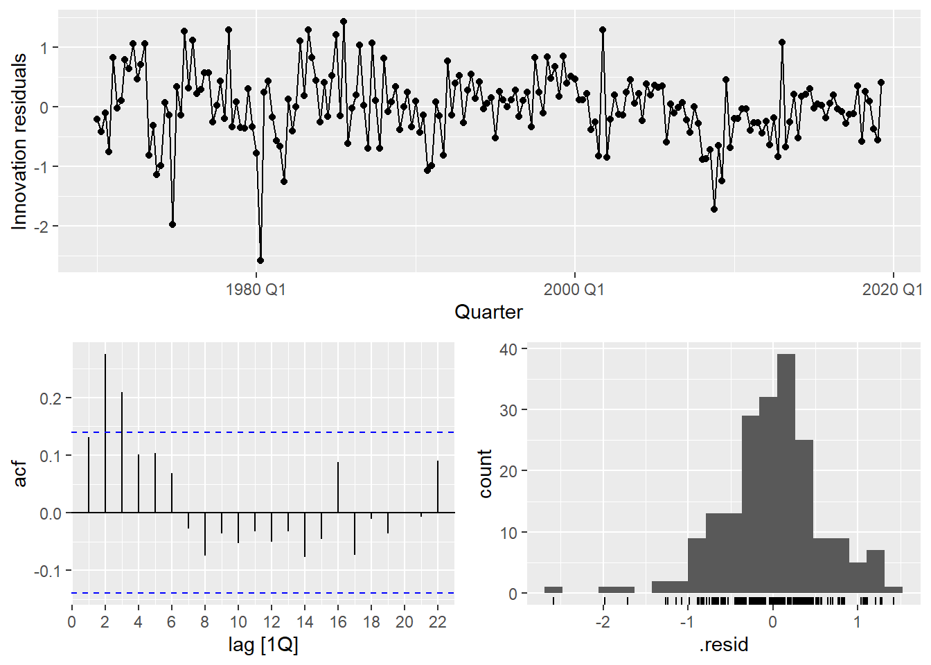
Code
- 1
- Extract the number of estimated parameters to use as degrees of freedom correction.
- 2
- A significant p-value indicates autocorrelated residuals — a sign the model is missing structure.
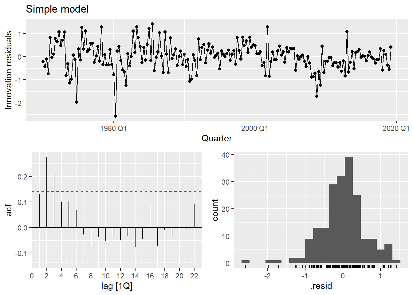
The residuals show clear autocorrelation. The simple model is not capturing all the dynamics of consumption. Let’s improve it.
4 Multiple Linear Regression
In practice, one predictor is rarely sufficient. The multiple linear regression model is:
y_t = \beta_0 + \beta_1 x_{1t} + \beta_2 x_{2t} + \cdots + \beta_k x_{kt} + \varepsilon_t
For us_change, a natural extension is:
y_{t, \text{Cons.}} = \beta_0 + \beta_1 x_{t, \text{Inc.}} + \beta_2 x_{t, \text{Prod.}} + \beta_3 x_{t, \text{Sav.}} + \beta_4 x_{t, \text{Unemp.}} + \varepsilon_t
Code
us_change_fit_mult <- us_change |>
  model(
1    multiple = TSLM(Consumption ~ Income + Production + Savings + Unemployment)
  )

report(us_change_fit_mult)- 1
-
The formula syntax is the same as the simple linear regression: just add more predictors with
+.
Series: Consumption
Model: TSLM

Residuals:
     Min       1Q   Median       3Q      Max
-0.90555 -0.15821 -0.03608  0.13618  1.15471

Coefficients:
              Estimate Std. Error t value Pr(>|t|)
(Intercept)   0.253105   0.034470   7.343 5.71e-12 ***
Income        0.740583   0.040115  18.461  < 2e-16 ***
Production    0.047173   0.023142   2.038   0.0429 *
Savings      -0.052890   0.002924 -18.088  < 2e-16 ***
Unemployment -0.174685   0.095511  -1.829   0.0689 .
---
Signif. codes:  0 '***' 0.001 '**' 0.01 '*' 0.05 '.' 0.1 ' ' 1

Residual standard error: 0.3102 on 193 degrees of freedom
Multiple R-squared: 0.7683, Adjusted R-squared: 0.7635
F-statistic:   160 on 4 and 193 DF, p-value: < 2.22e-16
4.0.1 Comparing simple vs. multiple
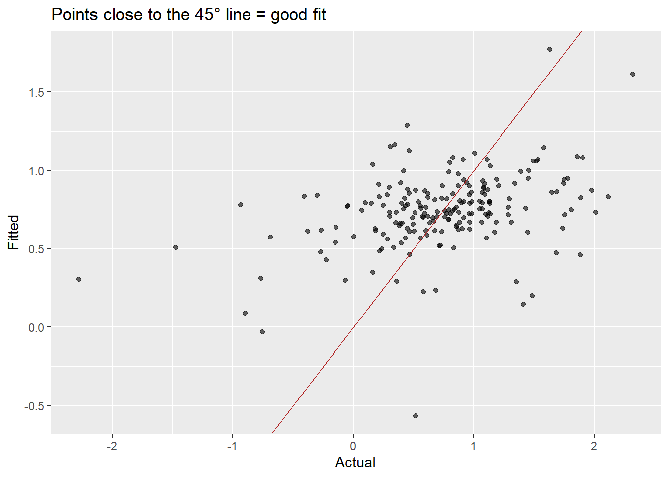
Grey line = actual consumption; colored line = fitted values. The multiple model tracks the data much more closely.
Points closer to the 45° line indicate better fit. The multiple model shows a much tighter cloud.
Code
bind_rows(
augment(us_change_fit_simple) |>
features(.resid, ljung_box, lag = 10, dof = 2) |>
mutate(.model = "Simple"),
augment(us_change_fit_mult) |>
features(.resid, ljung_box, lag = 10, dof = 5) |>
mutate(.model = "Multiple")
) |>
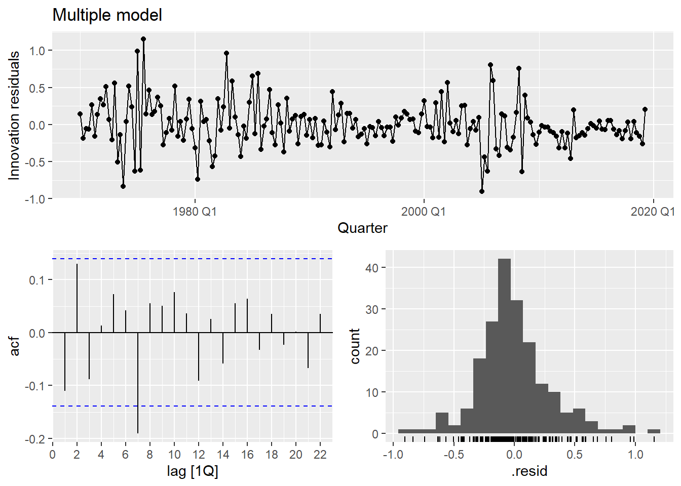
select(.model, lb_stat, lb_pvalue)The multiple model substantially improves fit (\bar{R}^2 goes from ~0.15 to ~0.75) and the residuals look much closer to white noise.
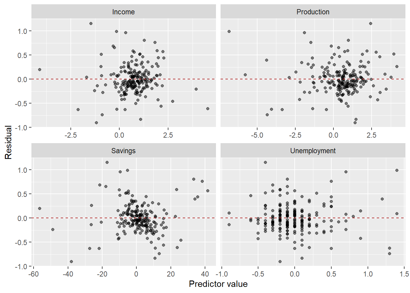
The residuals vs. predictors plot is a useful diagnostic specific to multiple regression. If any panel shows a systematic pattern (curve, fan shape), it suggests a missing nonlinear term or interaction involving that predictor.
5 Predictor Selection
With k potential predictors, there are 2^k possible models. We need a principled way to choose among them.
Do not use in-sample R^2 for selection. Adding any predictor, even a random one, increases R^2. We need measures that penalize model complexity.
The three standard criteria available from glance() in fable:
- Adjusted \bar{R}^2: penalizes for additional parameters. Maximize it.
- AIC (Akaike Information Criterion): -2\log L + 2k. Minimize it. Optimizes predictive performance.
- AICc: AIC corrected for small samples. Prefer this over AIC for time series.
- BIC (Bayesian Information Criterion): -2\log L + k \log T. Minimize it. BIC penalizes complexity more heavily and tends to select smaller models than AICc.
Code
glance(us_change_fit_mult) |>
  select(adj_r_squared, AIC, AICc, BIC)
5.0.1 Search strategies
Fit all possible models and compare:
Code
us_change_fit_select <- us_change |>
  model(
    m1 = TSLM(Consumption ~ Income),
    m2 = TSLM(Consumption ~ Income + Production),
    m3 = TSLM(Consumption ~ Income + Savings),
    m4 = TSLM(Consumption ~ Income + Unemployment),
    m5 = TSLM(Consumption ~ Income + Production + Savings),
    m6 = TSLM(Consumption ~ Income + Production + Unemployment),
    m7 = TSLM(Consumption ~ Income + Savings + Unemployment),
    m8 = TSLM(Consumption ~ Income + Production + Savings + Unemployment)
  )

us_change_fit_select |>
  glance() |>
  select(.model, adj_r_squared, AIC, AICc, BIC) |>
  arrange(AICc)
Start with the full model and remove predictors one at a time:
Code
us_change |>
  model(
    full  = TSLM(Consumption ~ Income + Production + Savings + Unemployment),
    drop1 = TSLM(Consumption ~ Income + Production + Savings),
    drop2 = TSLM(Consumption ~ Income + Production + Unemployment),
    drop3 = TSLM(Consumption ~ Income + Savings + Unemployment),
    drop4 = TSLM(Consumption ~ Production + Savings + Unemployment)
  ) |>
  glance() |>
  select(.model, adj_r_squared, AICc, BIC) |>
  arrange(AICc)
Start with the intercept-only model and add predictors one at a time:
Code
# Step 1: which single predictor is best?
us_change |>
  model(
    f1 = TSLM(Consumption ~ Income),
    f2 = TSLM(Consumption ~ Production),
    f3 = TSLM(Consumption ~ Savings),
    f4 = TSLM(Consumption ~ Unemployment)
  ) |>
  glance() |>
  select(.model, AICc) |>
  arrange(AICc)
Code
# Step 2: add a second predictor to the best single-predictor model
us_change |>
  model(
    f1  = TSLM(Consumption ~ Savings),
    f12 = TSLM(Consumption ~ Savings + Income),
    f13 = TSLM(Consumption ~ Savings + Production),
    f14 = TSLM(Consumption ~ Savings + Unemployment)
  ) |>
  glance() |>
  select(.model, AICc) |>
  arrange(AICc)
TipAICc vs. BIC: which one to use?
Both penalize model complexity, but differently:
- AICc minimizes expected out-of-sample prediction error. It tends to select slightly larger models.
- BIC is consistent: as T \to \infty, it will select the true model (if it’s in the candidate set). It penalizes more heavily and selects smaller models.
In forecasting contexts, AICc is generally preferred because we care more about predictive accuracy than model parsimony per se. When they disagree, consider whether interpretability or predictive accuracy is the primary goal.
5.1 Multicollinearity
Predictor selection and multicollinearity are closely linked. Even after running all-subsets or stepwise search, the selected model may still include predictors that are highly correlated with each other — and that creates problems that no information criterion will automatically flag.
When two or more predictors are highly correlated, we have multicollinearity. It does not bias the OLS estimates, but it inflates the variance of the coefficients, making them unstable and hard to interpret.
- In the extreme case of perfect collinearity (x_1 = c \cdot x_2), the model is unidentified: infinitely many solutions minimize SSR.
- In practice, collinearity is a matter of degree, not a binary condition.
- Warning signs: coefficients with unexpected signs, large standard errors, a significant F-test alongside non-significant individual t-tests.
5.1.1 Detecting multicollinearity: VIF
The Variance Inflation Factor (VIF) measures how much the variance of \hat{\beta}_j is inflated by its correlation with the other predictors:
\text{VIF}_j = \frac{1}{1 - R_j^2}
where R_j^2 is the R^2 obtained by regressing x_j on all the other predictors — a measure of how well one predictor can be linearly predicted by the rest.
- \text{VIF} = 1: no collinearity with other predictors.
- \text{VIF} \in (1, 5): moderate — generally acceptable.
- \text{VIF} > 5: concerning, examine carefully.
- \text{VIF} > 10: severe — take action.
A quick visual check: if the ggpairs scatter matrix shows strong correlations between predictors (not between a predictor and y), multicollinearity is likely present. The VIF quantifies exactly how severe that problem is.
5.1.2 What to do about multicollinearity
The answer depends critically on your goal.
- If your goal is forecasting — which is ours — multicollinearity is largely harmless. The individual \hat{\beta}’s may be unstable, but their joint contribution to \hat{y}_t is still well estimated. The model can produce excellent forecasts even when coefficients are hard to interpret individually.
The one scenario where multicollinearity does hurt forecasting is if the correlation structure among predictors breaks down in the future — i.e., predictors that moved together historically start moving independently. In that case, the model never learned their individual effects well enough to adapt.
- If your goal is inference — understanding the isolated effect of each predictor — multicollinearity is a real problem and should be addressed:
- Drop one of the correlated predictors — keep the one with stronger theoretical justification or cleaner interpretability.
- Combine them — create a composite index, take a ratio, or use the first principal component of the correlated group.
- Use penalized regression (Ridge, Lasso) — these accept a small bias in exchange for substantially lower variance. Outside this course’s scope, but worth knowing.
6 Forecasting with Regression
Before we can forecast y_t with regression, we need to ask: what do we do with the predictors?
With univariate models, forecast(h = n) was sufficient — the model only needed its own history. Now the model needs future values of x_t to produce a forecast of y_t.
What changes across the three forecasting types is precisely what values we assign to the predictors:
- Ex-ante: we forecast the predictors first, then use those forecasts as inputs.
- Ex-post: we use the actual realized values of the predictors.
- Scenario-based: we construct hypothetical values for the predictors.
6.1 Three types of regression forecasts
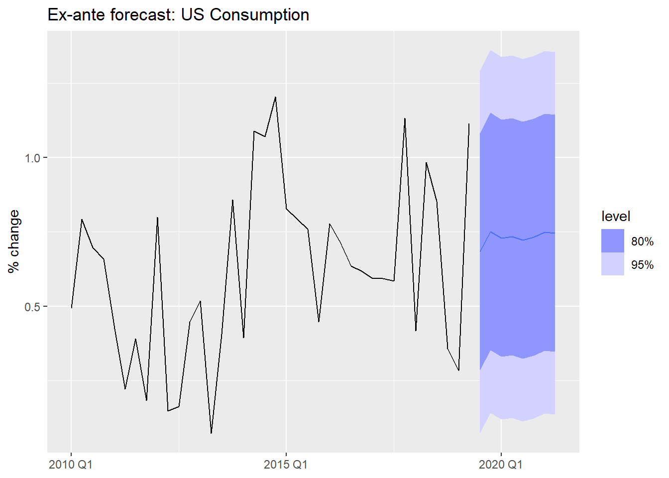
Ex-ante forecasts use only information available at the time the forecast is made. The predictors must themselves be forecasted.
This is the “true” forecast — it is what you would actually produce in a real deployment.
Code
us_change_future <- us_change |>
1  pivot_longer(-c(Quarter, Consumption), names_to = "variable") |>
2  model(arima = ARIMA(value)) |>
3  forecast(h = 8) |>
4  as_tsibble() |>
  select(-c(.model, value)) |>
5  pivot_wider(names_from = variable, values_from = .mean)

us_change_fit_mult |>
  forecast(new_data = us_change_future) |>
  autoplot(us_change |> filter_index("2010 Q1" ~ .)) +
  labs(title = "Ex-ante forecast: US Consumption",
y = "% change", x = NULL)- 1
-
Pivot to long format — each predictor becomes a separate series keyed by
variable. - 2
-
A single
model()call fits an ARIMA to each predictor automatically. - 3
-
A single
forecast()produces 8-step-ahead forecasts for all predictors simultaneously. - 4
-
Convert back to tsibble — required by
forecast()when passed asnew_data. - 5
- Pivot back to wide so each predictor has its own column, matching the structure expected by the regression model.
Ex-post forecasts use actual realized values of the predictors. The forecast variable y_t is still unknown, but we feed in the true future x_t values.
These are not “real” forecasts — they are used to evaluate the regression model in isolation, removing predictor forecast error from the evaluation.
Code
# Use filter_index to create a train/test split
us_change_train <- us_change |>
  filter_index(. ~ "2017 Q4")

us_change_test <- us_change |>
  filter_index("2018 Q1" ~ .)

us_change_fit_expost <- us_change_train |>
  model(
    multiple = TSLM(Consumption ~ Income + Production + Savings + Unemployment)
  )

# Ex-post: we supply actual future predictor values
us_change_fit_expost |>
  forecast(new_data = us_change_test) |>
  autoplot(us_change |> filter_index("2014 Q1" ~ .)) +
  labs(title = "Ex-post forecast: actual predictor values used",
       y = "% change", x = NULL)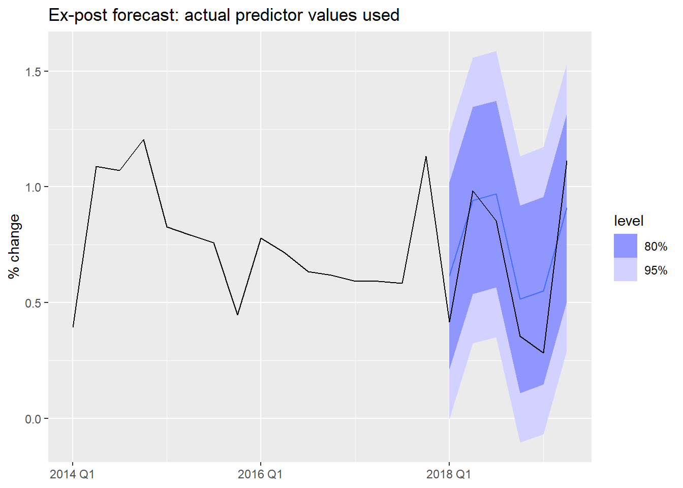
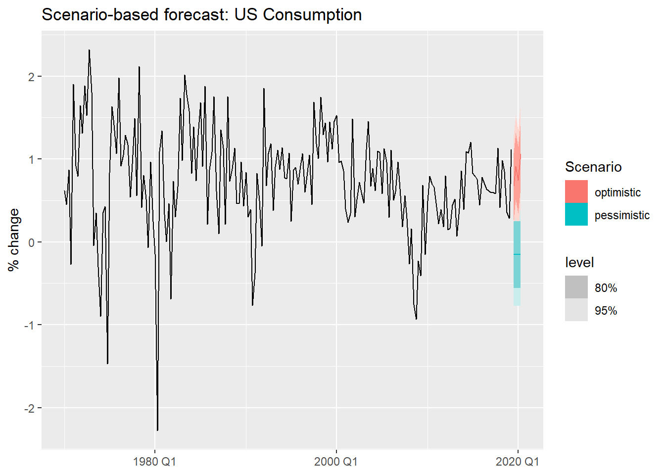
Scenario-based forecasts construct hypothetical future values for the predictors and ask: what would consumption look like under each scenario?
These are especially useful for stress-testing and strategic planning.
Code
us_change_fit_scen <- us_change |>
1  model(TSLM(Consumption ~ Income + Savings + Unemployment))

us_change_scenarios <- scenarios(
  optimistic = new_data(us_change, 4) |>
2    mutate(Income = c(0.5, 0.8, 0.6, 1.0),
           Savings = c(0.1, -0.2, 0.1, -0.1),
           Unemployment = -0.1),
  pessimistic = new_data(us_change, 4) |>
3    mutate(Income = -0.5,
           Savings = -0.4,
           Unemployment = 0.2),
4  names_to = "Scenario"
)

us_change |>
  autoplot(Consumption) +
5  autolayer(forecast(us_change_fit_scen, new_data = us_change_scenarios)) +
  labs(title = "Scenario-based forecast: US Consumption",
y = "% change", x = NULL)- 1
- We fit a simpler model using only the three predictors with clearest economic interpretation.
- 2
- Optimistic scenario: income grows steadily, savings fluctuate mildly, unemployment falls slightly.
- 3
- Pessimistic scenario: income contracts, savings decline, unemployment rises.
- 4
-
names_tolabels each scenario in the output, making it easy to distinguish them in the plot. - 5
-
autolayer()overlays the scenario forecasts on the historical series without requiring matching key structures.
7 Useful Predictors
We have seen regression with exogenous variables. But can TSLM() also handle the patterns we identified in Module 1 — trend and seasonality?
Yes — through specially constructed predictors built directly into the formula.
We will illustrate with quarterly beer production in Australia.
Code
beer <- aus_production |>
  filter(year(Quarter) >= 1992) |>
  select(Quarter, Beer)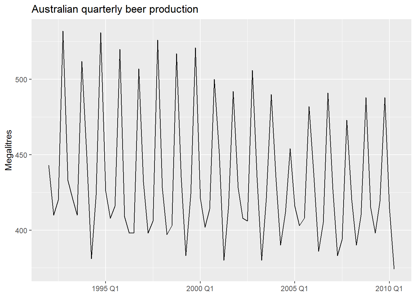
7.1 Seasonal dummy variables
To capture seasonality in a regression, we use dummy variables — binary indicators that take the value 1 for a specific season and 0 otherwise.
- A quarterly series has 4 seasons. How many dummies do we need?
- Not 4 — only 3. One season is left as the baseline (absorbed into the intercept).
- Including all 4 would create perfect collinearity with the intercept: the dummy variable trap.
This is analogous to a cross-sectional dummy: to distinguish male/female, you only need one binary variable — one category is always implicit in the intercept.
7.1.1 What the dummies look like
Code
beer |>
  mutate(
    t  = row_number(),
    Q2 = if_else(quarter(Quarter) == 2, 1L, 0L),
    Q3 = if_else(quarter(Quarter) == 3, 1L, 0L),
    Q4 = if_else(quarter(Quarter) == 4, 1L, 0L)
  ) |>
  head(8)
The dummy variable trap: if you create dummies for all m seasons and include an intercept, you have perfect multicollinearity. Always use m - 1 dummies. TSLM() handles this automatically with season().
7.2 Trend and seasonal dummies in R
TSLM() provides two built-in terms:
trend()— a deterministic linear trend: \beta_1 t where t = 1, 2, \ldots, T.season()— m - 1 seasonal dummy variables, with the first season as baseline.
Code
beer_fit <- beer |>
  model(
1    TSLM(Beer ~ trend() + season())
  )

report(beer_fit)- 1
-
trend()adds a linear time index;season()adds quarterly dummies automatically.
Series: Beer
Model: TSLM

Residuals:
     Min       1Q   Median       3Q      Max
-42.9029  -7.5995  -0.4594   7.9908  21.7895

Coefficients:
               Estimate Std. Error t value Pr(>|t|)
(Intercept)   441.80044    3.73353 118.333  < 2e-16 ***
trend()        -0.34027    0.06657  -5.111 2.73e-06 ***
season()year2 -34.65973    3.96832  -8.734 9.10e-13 ***
season()year3 -17.82164    4.02249  -4.430 3.45e-05 ***
season()year4  72.79641    4.02305  18.095  < 2e-16 ***
---
Signif. codes:  0 '***' 0.001 '**' 0.01 '*' 0.05 '.' 0.1 ' ' 1

Residual standard error: 12.23 on 69 degrees of freedom
Multiple R-squared: 0.9243, Adjusted R-squared: 0.9199
F-statistic: 210.7 on 4 and 69 DF, p-value: < 2.22e-16
NoteWhat about more complex seasonality? Fourier terms
For series with multiple seasonal periods or very long seasons (daily, hourly data), season() becomes impractical — the number of dummies grows too large. An alternative is Fourier terms: pairs of sine and cosine waves that approximate the seasonal pattern with far fewer parameters.
TSLM() supports this via fourier(K), where K controls how many Fourier pairs are included. We will cover this properly in Module 4 when we deal with complex seasonality.
Code
beer_fit |>
  gg_tsresiduals()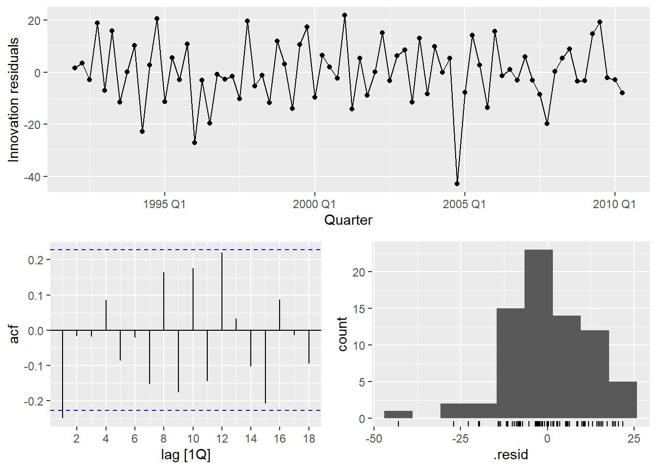
There is a notable outlier in Q2 1994. We can detect it formally and then handle it with an intervention variable.
7.3 Intervention Variables and Outliers
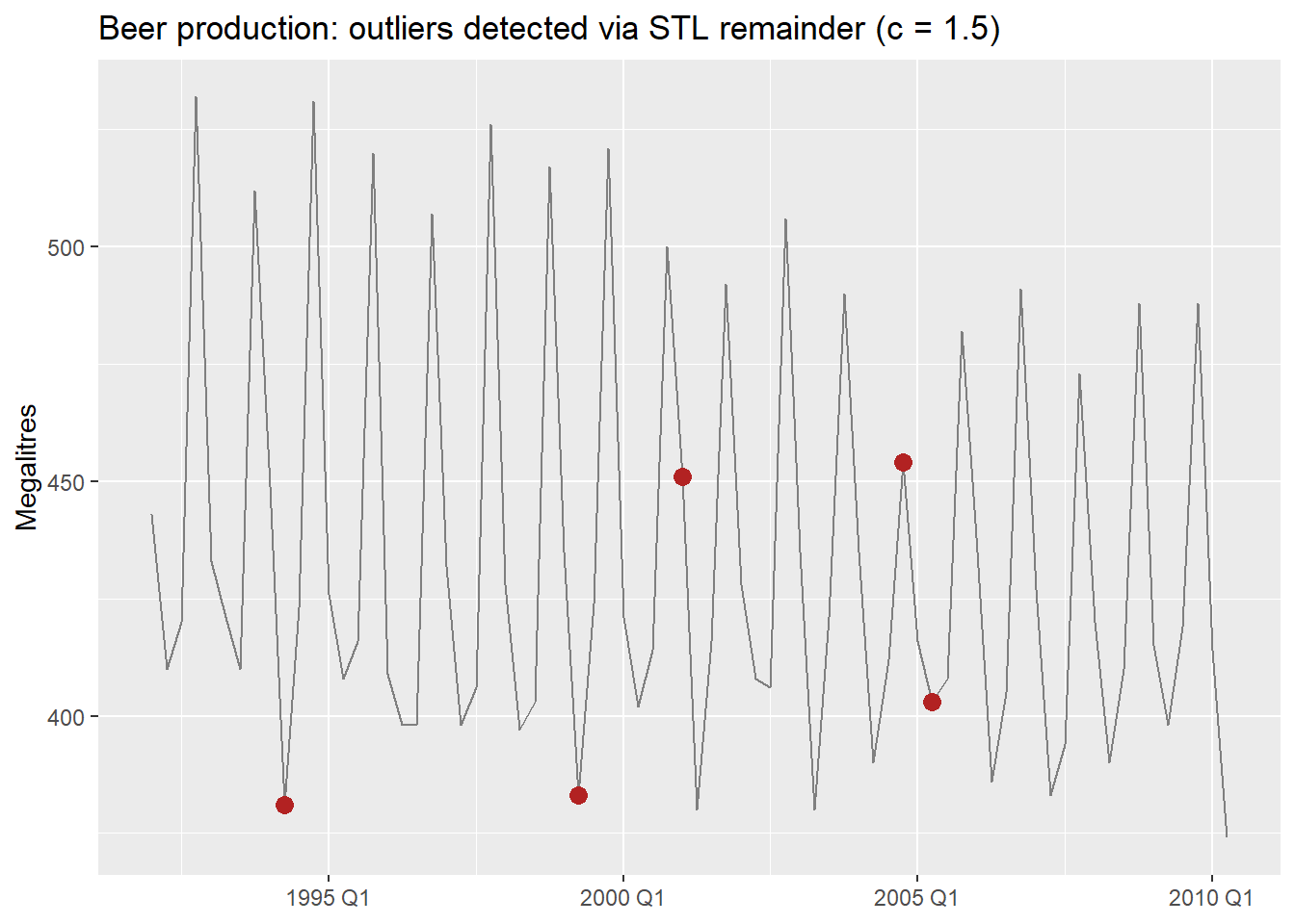
Rather than eyeballing the residual plot, we can detect outliers formally — the same way we did in the practical issues document. The key idea is that applying the IQR rule directly to the raw series does not work in time series: a series with trend has naturally increasing values, so later observations always look “large” even when they are perfectly normal.
The fix: decompose first, then apply IQR to the remainder. For beer, which has strong known seasonality, we use a full STL decomposition — including the seasonal component — so only genuine anomalies end up in the remainder1.
Code
beer_dcmp <- beer |>
  model(
1    stl = STL(Beer ~ trend() + season(), robust = TRUE)
  ) |>
  components()

beer_outliers <- beer_dcmp |>
  select(Quarter, remainder) |>
  mutate(
    Q1  = quantile(remainder, 0.25),
    Q3  = quantile(remainder, 0.75),
    IQR = Q3 - Q1,
2    lower_15 = Q1 - 1.5 * IQR,
    upper_15 = Q3 + 1.5 * IQR,
3    lower_3  = Q1 - 3   * IQR,
    upper_3  = Q3 + 3   * IQR,
    outlier_15 = remainder < lower_15 | remainder > upper_15,
    outlier_3  = remainder < lower_3  | remainder > upper_3
  )

beer_outliers |>
  filter(outlier_15) |>
select(Quarter, remainder, outlier_15, outlier_3)- 1
-
Full STL with both trend and season — for a strongly seasonal series like
beer, this prevents normal seasonal variation from being flagged as anomalies. - 2
- Standard threshold (c = 1.5): flags moderate outliers.
- 3
- Stricter threshold (c = 3): flags only extreme observations. Use this when you want to be conservative.
7.3.1 Types of intervention variables
In regression, rather than removing the outlier and imputing, we model it explicitly with a dummy variable. This keeps all observations and lets the model account for the anomaly without distorting the other coefficients.
- Spike variable: 1 for a single anomalous period, 0 everywhere else. Captures a one-off shock.
- Level shift variable: 0 before an event, 1 from the event onward. Captures a permanent change in level.
- Ramp variable: 0 before an event, then increasing linearly. Captures a gradual structural shift.
Code
- 1
- Spike: 1 only in 1994 Q2, captures the single anomalous quarter.
- 2
- Level shift: 1 from year 2000 onward, allows a different intercept from that point.
Series: Beer
Model: TSLM

Residuals:
     Min       1Q   Median       3Q      Max
-42.7196  -6.9594  -0.7748   8.0050  21.5292

Coefficients:
              Estimate Std. Error t value Pr(>|t|)
(Intercept)   442.6530     3.8050 116.336  < 2e-16 ***
trend()        -0.3730     0.1285  -2.902  0.00501 **
season()year2 -33.3328     3.9745  -8.387 4.84e-12 ***
season()year3 -17.8072     3.9716  -4.484 2.95e-05 ***
season()year4  72.8436     3.9773  18.315  < 2e-16 ***
spike_Q2_1994 -24.5904    12.5547  -1.959  0.05432 .
level_2000      0.6182     5.5264   0.112  0.91127
---
Signif. codes:  0 '***' 0.001 '**' 0.01 '*' 0.05 '.' 0.1 ' ' 1

Residual standard error: 12.07 on 67 degrees of freedom
Multiple R-squared: 0.9284, Adjusted R-squared: 0.922
F-statistic: 144.9 on 6 and 67 DF, p-value: < 2.22e-16
We will revisit outlier handling in Module 4, where we cover robust methods and automatic outlier detection. Intervention variables are the regression-world equivalent of those techniques — explicit rather than automatic.
8 Nonlinear Regression
We established earlier that linear in the parameters does not mean a straight line. Here are the three most practically useful nonlinear forms — all estimable by OLS.
8.1 Log Transformations
What changes relative to a standard linear regression is not the estimation method — it is the interpretation of the coefficients.
| Model | Equation | Interpretation of \hat{\beta}_1 |
|---|---|---|
| Lin-lin (standard) | y_t = \beta_0 + \beta_1 x_t + \varepsilon_t | 1-unit \uparrow x → \hat{\beta}_1-unit change in y |
| Log-log (elasticity) | \log y_t = \beta_0 + \beta_1 \log x_t + \varepsilon_t | 1% \uparrow x → \hat{\beta}_1% change in y |
| Log-lin (semi-elasticity) | \log y_t = \beta_0 + \beta_1 x_t + \varepsilon_t | 1-unit \uparrow x → 100\hat{\beta}_1% change in y |
| Lin-log | y_t = \beta_0 + \beta_1 \log x_t + \varepsilon_t | 1% \uparrow x → \hat{\beta}_1/100-unit change in y |
NoteWhat about other transformations?
These interpretations hold cleanly only for the natural logarithm (\ln). Two common alternatives:
Logarithm in a different base (e.g., \log_{10}): the coefficient is scaled by \ln(b) where b is the base. The elasticity interpretation is preserved in shape but the numeric value changes — an unnecessary complication. Stick with \ln.
Box-Cox (\lambda \neq 0, 1): the response is on the scale \frac{y^\lambda - 1}{\lambda}, which has no clean verbal interpretation. Box-Cox is better used as a pre-processing transformation to stabilize variance before modeling (as in Module 1) than inside a regression model where you need to interpret the coefficients.
8.2 Piecewise Linear Trends
When the trend changes slope at one or more points in time, a piecewise linear model fits separate linear segments joined at knots.
We use the Boston Marathon winning times — a series with clear structural breaks.
Code
boston_men <- boston_marathon |>
  filter(Event == "Men's open division") |>
  mutate(Minutes = as.numeric(Time) / 60)

boston_men |>
  autoplot(Minutes) +
  labs(title = "Boston Marathon: men's open division winning times",
       y = "Minutes", x = NULL)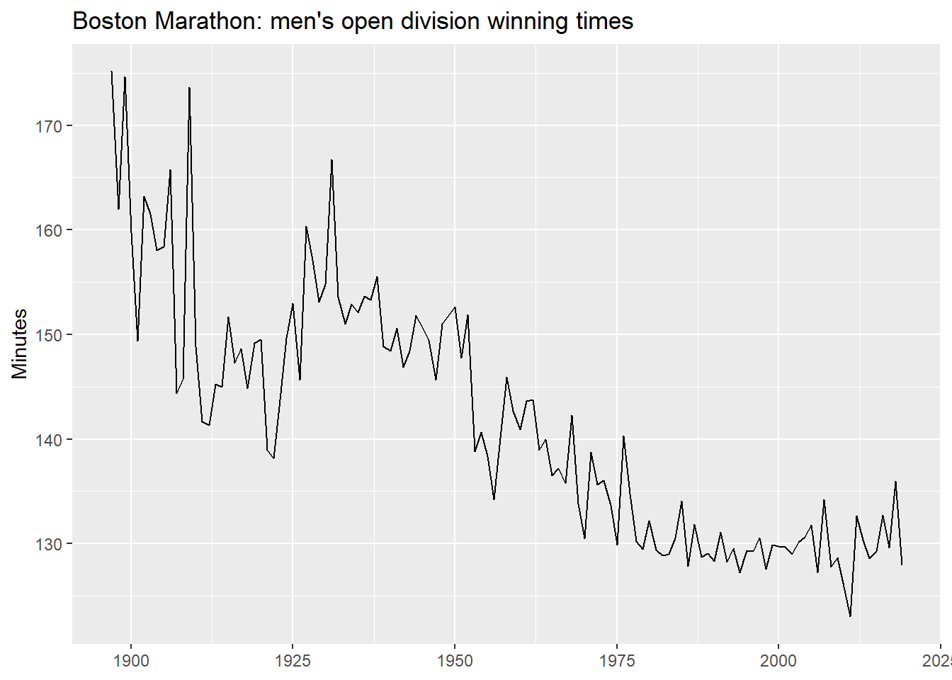
8.2.1 A linear trend first
What does a single linear trend produce on this data?
Code
boston_fit_linear <- boston_men |>
  model(linear = TSLM(Minutes ~ trend()))

boston_men |>
  autoplot(Minutes, color = "grey60") +
  geom_line(
    data = fitted(boston_fit_linear),
    aes(y = .fitted), color = "#0072B2"
  ) +
  autolayer(forecast(boston_fit_linear, h = 10),
            alpha = 0.5, level = 95) +
  labs(title = "Boston Marathon: linear trend",
       y = "Minutes", x = NULL)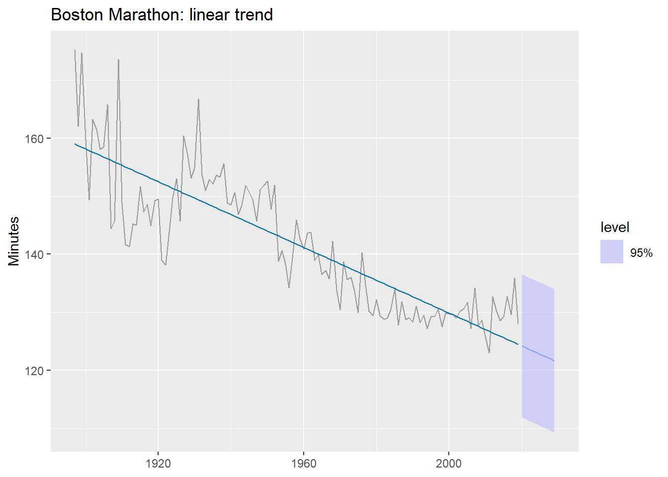
The forecast predicts times will keep falling indefinitely — eventually reaching zero. A single linear trend is the wrong functional form here.
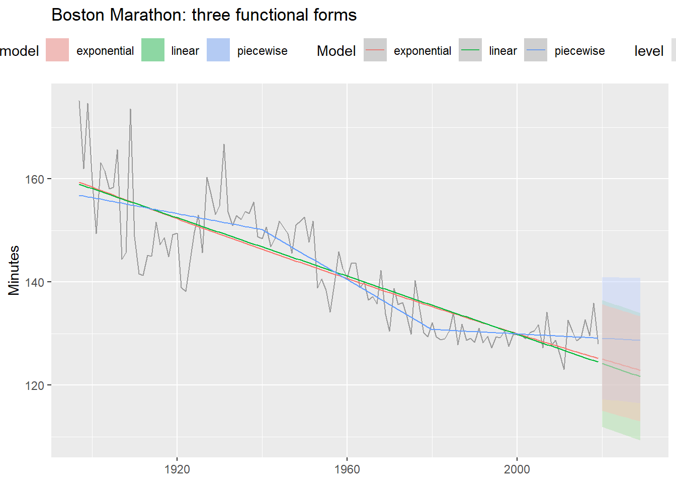
8.2.2 Three functional forms
Code
boston_fit <- boston_men |>
  model(
    linear      = TSLM(Minutes ~ trend()),
1    exponential = TSLM(log(Minutes) ~ trend()),
2    piecewise   = TSLM(Minutes ~ trend(knots = c(1940, 1980)))
  )

boston_men |>
  autoplot(Minutes, color = "grey60") +
  geom_line(
    data = fitted(boston_fit),
    aes(y = .fitted, color = .model)
  ) +
  autolayer(forecast(boston_fit, h = 10),
            alpha = 0.4, level = 95) +
  labs(title = "Boston Marathon: three functional forms",
       y = "Minutes", x = NULL, color = "Model") +
theme(legend.position = "top")- 1
- Log-transformed response: assumes times decrease at a declining rate.
- 2
-
knotsspecify the years where the slope is allowed to change.
Code
accuracy(boston_fit) |>
  select(.model, RMSE, MAE, MAPE) |>
  arrange(MAPE)
8.2.3 The knot selection problem
A key limitation of piecewise regression: we must choose the knots ourselves. Different choices can produce very different forecasts, even when in-sample fit looks similar.
Code
boston_fit_knots <- boston_men |>
  model(
    k1 = TSLM(Minutes ~ trend(knots = c(1940, 1980))),
    k2 = TSLM(Minutes ~ trend(knots = c(1915, 1950))),
    k3 = TSLM(Minutes ~ trend(knots = c(1950, 1970, 1990)))
  )

boston_men |>
  autoplot(Minutes, color = "grey60") +
  geom_line(
    data = fitted(boston_fit_knots),
    aes(y = .fitted, color = .model)
  ) +
  autolayer(forecast(boston_fit_knots, h = 10),
            alpha = 0.4, level = 95) +
  labs(title = "Different knots → very different forecasts",
       y = "Minutes", x = NULL, color = "Model") +
  theme(legend.position = "top")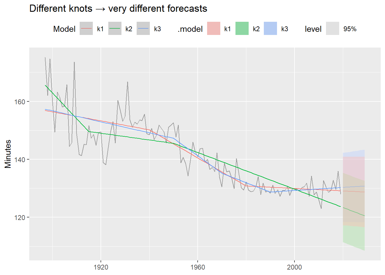
These models fit the historical data similarly well — but their forecasts diverge dramatically. Always inspect the forecast, not just the in-sample fit. This is one motivation for Prophet (Module 4), which detects changepoints automatically from the data rather than requiring manual specification.
9 Summary
| Model | Formula | When to use |
|---|---|---|
| Simple TSLM | TSLM(y ~ x) |
One meaningful exogenous predictor; baseline |
| Multiple TSLM | TSLM(y ~ x1 + x2 + ...) |
Several predictors; check multicollinearity |
| Trend + season | TSLM(y ~ trend() + season()) |
Deterministic trend and/or fixed seasonality |
| Interventions | TSLM(y ~ ... + spike + shift) |
Known outliers or structural breaks |
| Log-log | TSLM(log(y) ~ log(x)) |
Elasticity relationships |
| Log-lin | TSLM(log(y) ~ trend()) |
Exponential growth/decay |
| Piecewise | TSLM(y ~ trend(knots = c(...))) |
Trend with known structural breaks |
Key takeaways:
- Regression adds external context that purely univariate models cannot capture.
- Correlation ≠ causality — always.
- Residual diagnostics are not optional: autocorrelated residuals invalidate inference.
- Multicollinearity hurts interpretation, but usually not forecast accuracy.
- For forecasting with regression you must decide what to do with future predictor values: ex-ante, ex-post, or scenario-based.
- More flexible functional forms improve fit but require careful inspection of the forecasts.
Coming up in 3.3: Dynamic regression — what happens when we let the error term \varepsilon_t follow an ARIMA process instead of assuming white noise. This directly addresses the residual autocorrelation we saw in the simple model.
Footnotes
When seasonality is weak or absent,
season(period = 1)can be used to extract only the trend. See Practical Forecasting Issues for the full workflow including NA imputation.↩︎