The Forecasting Workflow using `fable`

Author

Pablo Benavides

Published

September 30, 2022

Modified

September 4, 2025

Introduction

0.1 Packages

It is recommended to load all the packages at the beginning of your file. We will be using the tidyverts ecosystem for the whole forecasting workflow.

library(tidyverse)
library(fpp3)
library(plotly)

Warning

Do not load unnecesary packages into your environment. It could lead to conflicts between functions and unwanted results.

1 Forecasting Workflow

1.1 Data

We will work with the Real Gross Domestic Product (GDP) for Mexico. The data is downloaded from FRED. The time series id is NGDPRNSAXDCMXQ.

1.1.1 Import data

gdp <- tidyquant::tq_get(
  x    = "NGDPRNSAXDCMXQ",
  get  = "economic.data",
  from = "1997-01-01"
)

gdp

# A tibble: 113 × 3
   symbol         date          price
   <chr>          <date>        <dbl>
 1 NGDPRNSAXDCMXQ 1997-01-01 3702398.
 2 NGDPRNSAXDCMXQ 1997-04-01 3896084.
 3 NGDPRNSAXDCMXQ 1997-07-01 3906063 
 4 NGDPRNSAXDCMXQ 1997-10-01 4038358.
 5 NGDPRNSAXDCMXQ 1998-01-01 4084304.
 6 NGDPRNSAXDCMXQ 1998-04-01 4134899.
 7 NGDPRNSAXDCMXQ 1998-07-01 4138200.
 8 NGDPRNSAXDCMXQ 1998-10-01 4146841.
 9 NGDPRNSAXDCMXQ 1999-01-01 4176243.
10 NGDPRNSAXDCMXQ 1999-04-01 4232280.
# ℹ 103 more rows

1.1.2 Wrangle data

There are some issues with our data:

It is loaded into a tibble object. We need to convert it to a tsibble.

Tip

We can use as_tsibble() to do so.

Our data is quarterly, but it is loaded in a YYYY-MM-DD format. We need to change it to a YYYY QQ format.

Tip

There are some functions that help us achieve this, such as

yearquarter()
yearmonth()
yearweek()
year()

depending on the time series’ period.

We will overwrite our data:

gdp <- gdp |> 
  mutate(date = yearquarter(date)) |> 
  as_tsibble(
    index = date,
    key   = symbol
  )

gdp

Tip

We always need to specify the index argument, as it is our date variable.
The key argument is necessary whenever we have more than one time series in our data frame and is made up of one or more columns that uniquely identify each time series .

1.2 Train/Test Split

We will split our data in two sets: a training set, and a test set, in order to evaluate our forecasts’ accuracy.

gdp_train <- gdp |> 
  filter_index(. ~ "2021 Q4")

gdp_train

Note

For all our variables, it is strongly recommended to follow the same notation process, and write our code using snake_case. Here, we called our data gdp, therefore, all the following variables will be called starting with gdp_¹, such as gdp_train for our training set.

1.3 Visualization and EDA

When performing time series analysis/forecasting, one of the first things to do is to create a time series plot.

p <- gdp_train |> 
  autoplot(price) +
  labs(
    title = "Time series plot of the Real GDP for Mexico",
    y = "GDP"
  )
 
ggplotly(p, dynamicTicks = TRUE) |> 
  rangeslider()

Our data exhibits an upward linear trend (with some economic cycles), and strong yearly seasonality.

We will explore it further with a season plot.

gdp_train |> 
  gg_season(price) |> 
  ggplotly()

1.3.1 TS Decomposition

gdp_train |> 
  model(stl = STL(price, robust = TRUE)) |> 
  components() |> 
  autoplot() |> 
  ggplotly()

The STL decomposition shows that the variance of the seasonal component has been increasing. We could try using a log transformation to counter this.

gdp_train |> 
  autoplot(log(price)) +
  ggtitle("Log of the Real GDP of Mexico")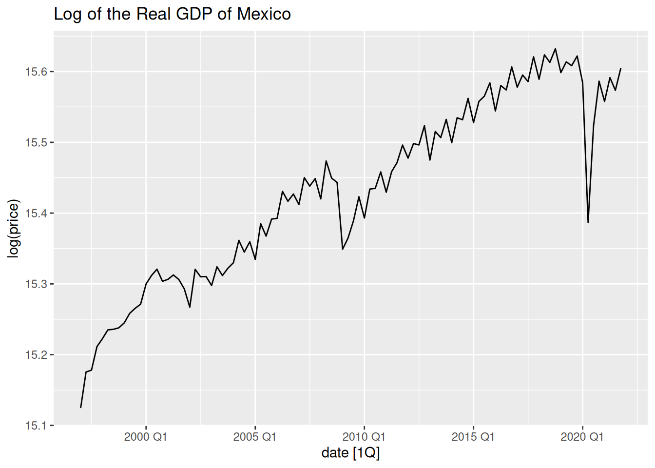

gdp_train |> 
  model(stl = STL(log(price) ~ season(window = "periodic"), robust = TRUE)) |> 
  components() |> 
  autoplot() |> 
  ggplotly()

1.4 Model Specification

We will fit two models to our time series: Seasonal Naïve, and the Drift model. We will also use the log transformation.

gdp_fit <- gdp_train |> 
  model(
    snaive = SNAIVE(log(price)),
    drift  = RW(log(price) ~ drift())
  )

Benchmark models

We have four different benchmark models that we’ll use to compare against the rest of the more complex models:

Mean (MEAN( <.y> ))
Naïve (NAIVE( <.y> ))
Seasonal Naïve (SNAIVE( <.y> ))
Drift (RW( <.y> ~ drift()))

where <.y> is just a placeholder for the variable to model.

Choose wisely which of these to use in each case, according to the exploratory analysis performed.

1.5 Residuals Diagnostics

1.5.1 Visual analysis

gdp_fit |> 
  select(snaive) |> 
  gg_tsresiduals() +
  ggtitle("Residuals Diagnostics for the Seasonal Naïve Model")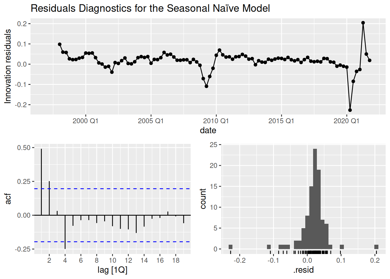

gdp_fit |> 
  select(drift) |> 
  gg_tsresiduals() +
  ggtitle("Residuals Diagnostics for the Drift Model")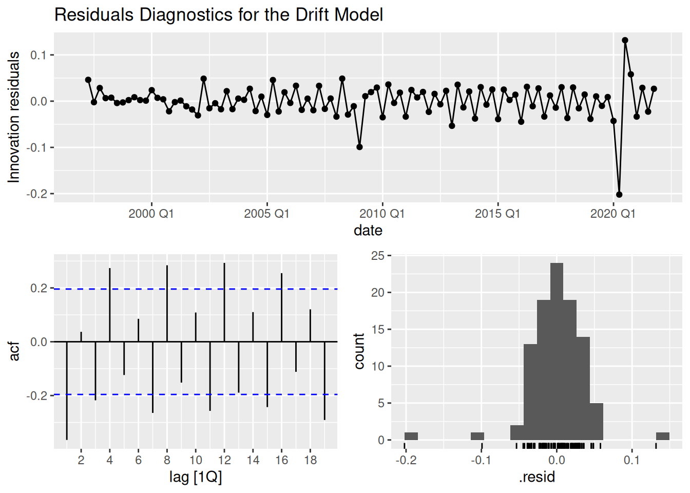

Tip

Here we expect to see:

A time series with no apparent patterns (no trend and/or seasonality), with a mean close to zero.
In the ACF, we’d expect no lags with significant autocorrelation.
Normally distributed residuals.

1.5.2 Portmanteau tests of autocorrelation

gdp_fit |> 
  augment() |> 
  features(.innov, ljung_box, lag = 24, dof = 0)

Residuals interpretation

Both models produce sub optimal residuals:

The SNAIVE correctly detects the seasonality, however, its residuals are still autocorrelated. Moreover, the residuals are not normally distributed.
The drift model doesn’t account for the seasonality, and their distribution is a little bit skewed.

Hence, we will perform our forecasts using the bootstrapping method.

We can compute some error metrics on the training set using the accuracy() function:

gdp_train_accu <- accuracy(gdp_fit) |> 
  arrange(MAPE)
gdp_train_accu |> 
  select(symbol:.type, MAPE, RMSE, MAE, MASE)

The accuracy() function

The accuracy() function can be used to compute error metrics in the training data, or in the test set. What differs is the data that is given to it:

For the training metrics, you need to use the mable (the table of models, that we usually store in _fit).
For the forecasting error metrics, we need the fable (the forecasts table, usually stored as _fc or _fcst), and the complete set of data (both the training and test set together).

For this analysis, we are focusing on the MAPE² metric. The drift model (2.47%) seems to have a better fit with the training set than the snaive model (3.24%).

1.6 Modeling using decomposition

We will perform a forecast using decomposition, to see if we can improve our results so far.

gdp_fit_dcmp <- gdp_train |> 
      model(
        stlf = decomposition_model(
          STL(log(price) ~ season(window = "periodic"), robust = TRUE),
          RW(season_adjust ~ drift())
        )
      )

gdp_fit_dcmp

Note on decomposition_model()

Remember, when using decomposition models, we need to do the following:

Specify what type of decomposition we want to use and customize it as needed.
Fit a model for the seasonally adjusted data; season_adjust.
Fit a model for the seasonal component. R uses a SNAIVE() model by default to model the seasonality. If you wish to model it using a different model, you have specify it.

The name of the seasonal component depends on the type of seasonality present in the time series. If it has a yearly seasonality, the component is called season_year. It could also be called season_week, season_day, and so on.

We can join this new model with the models we trained before. This way we can have them all in the same mable.

gdp_fit <- gdp_fit |> 
  left_join(gdp_fit_dcmp)

Joining with `by = join_by(symbol)`

1.6.1 Residuals diagnostics

gdp_fit |> 
  accuracy() |> 
  select(symbol:.type, MAPE, RMSE, MAE, MASE) |> 
  arrange(MAPE)

gdp_fit |> 
  select(stlf) |> 
  gg_tsresiduals()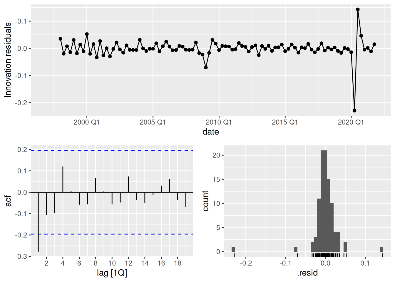

gdp_fit |> 
  augment() |> 
  features(.innov, ljung_box)

The MAPE seems to improve with this decomposition model. Also, the residual diagnostics do not show any seasonality present in them. However, the residuals are still autocorrelated, as the Ljung-Box test suggests.

1.7 Forecasting on the test set

Once we have our models, we can produce forecasts. We will forecast our test data and check our forecasts’ performance.

gdp_fc <- gdp_fit |> 
  forecast(h = gdp_h_fc) 

gdp_fc

gdp_fc |> 
  autoplot(gdp) +
  facet_wrap(~.model, ncol = 1)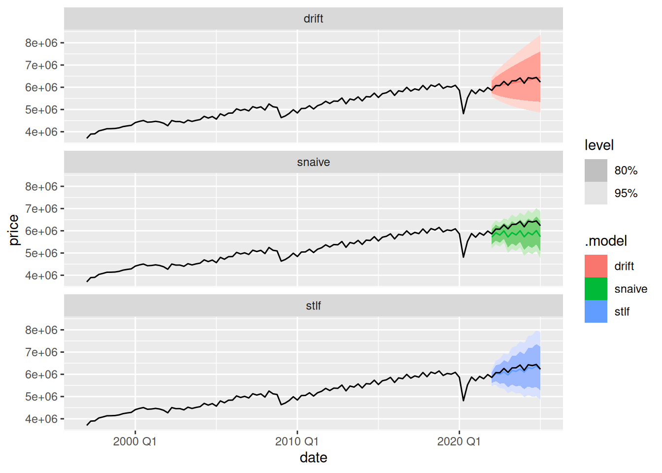

gdp_fc |> 
  filter(.model == "stlf") |> 
  autoplot(gdp)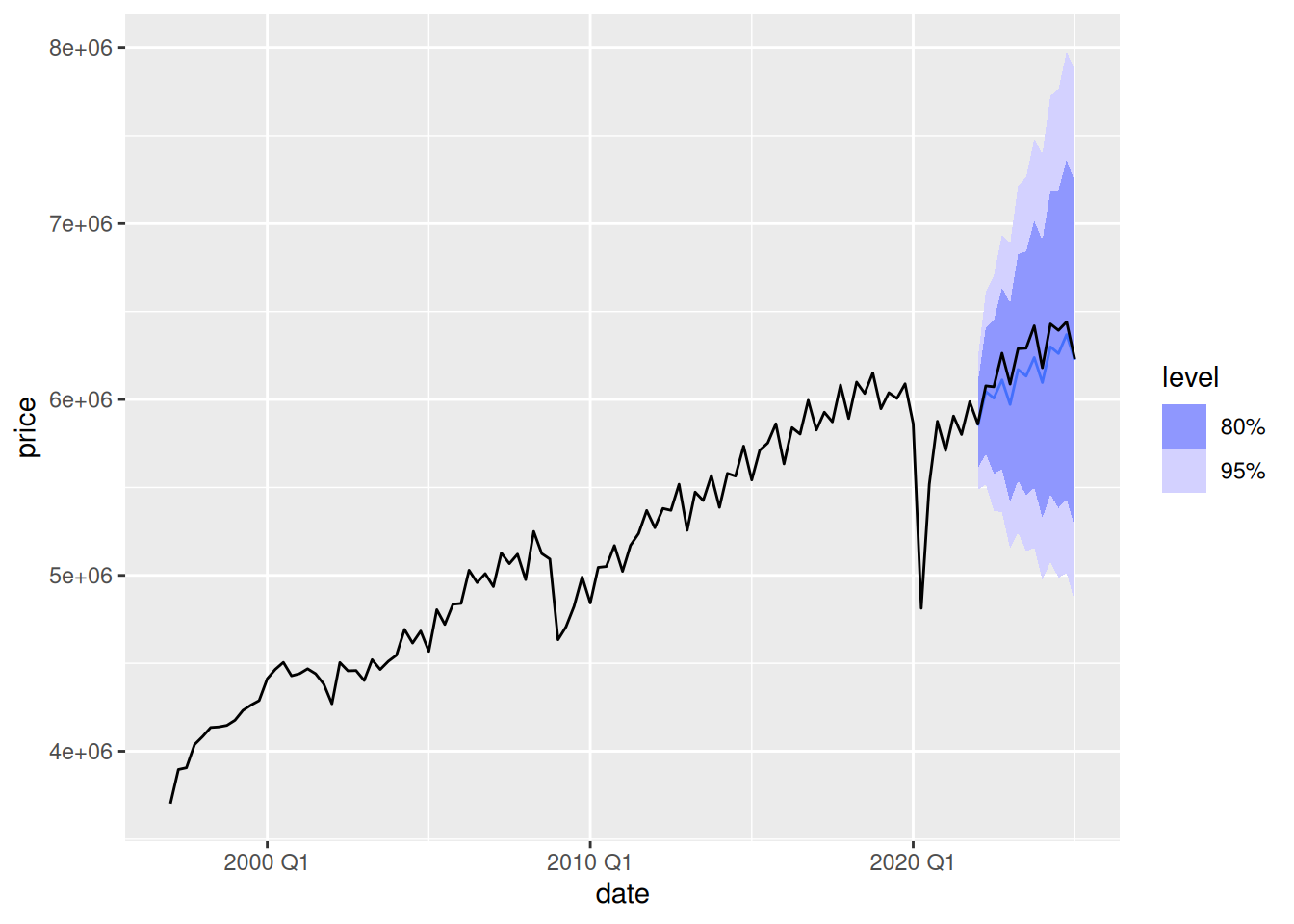

We now estimate the forecast errors:

gdp_fc |> 
  accuracy(gdp) |> 
  select(.model:.type, MAPE, RMSE, MAE, MASE) |> 
  arrange(MAPE)

1.8 Forecasting the future

We now refit our model using the whole dataset. We will only model the STL decomposition model, because the other two didn’t get a strong fit.

gdp_fit2 <- gdp |> 
  model(
    stlf = decomposition_model(
          STL(log(price) ~ season(window = "periodic"), robust = TRUE),
          RW(season_adjust ~ drift())
        )
  )
gdp_fit2

gdp_fc_fut <- gdp_fit2 |> 
  forecast(h = gdp_h_fc)
gdp_fc_fut

gdp_fc_fut |> 
  autoplot(gdp)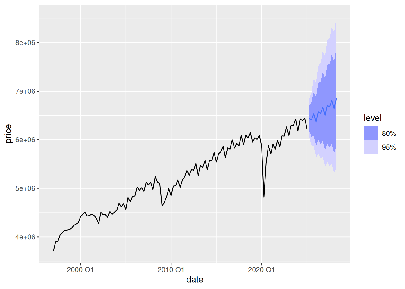

# save(gdp_fc_fut, file = "equipo1.RData")

Footnotes

This will make it very convenient when calling your variables. RStudio will display all the options starting with gdp_. We will usually use the following suffixes:
- _train: training set
- _fit: the mable (table of models)
- _aug: the augmented table with fitted values and residuals
- _dcmp: for the dable (decomposition table), containing the components and the seasonally adjusted series of a TS decomposition.
- _fc or _fcst: for the fable (forecasts table) that has our forecasts.
↩︎
The Mean Absolute Percentage Error is a percentage error metric widely used in professional environments.

Let

\[ e_t = y_t - \hat{y}_t \]

be the error or residual.

Then the MAPE would be computed as

\[ MAPE = \frac{1}{T}\sum_{t=1}^T|\frac{e_t}{y_t}| \].

↩︎