Complex Seasonality

Modified

May 8, 2026

Code

1library(plotly)

1: For interactive plots with dynamic ticks and range sliders.

Back in Module 3.3, we modeled electricity demand using daily aggregated data. Temperature explained the U-shaped relationship with demand, and day-type dummies captured the weekday/weekend pattern.

That model worked reasonably well — but it swept a fundamental problem under the rug: by aggregating to daily, we collapsed two distinct intra-day and intra-week cycles into a single, blunt average.

What we lost by aggregating

Daily demand is the sum of 48 half-hourly observations. When we aggregate, we lose:

The within-day pattern: morning ramp-up, midday plateau, evening peak, overnight trough
The within-week pattern: systematic differences across the seven days of the week

These are not noise — they are real, structured, forecastable signal.

1 The Data

1.1 From half-hourly to hourly

The vic_elec dataset records electricity demand in Victoria, Australia at 30-minute intervals, from 2012 to 2014. We aggregate to hourly to preserve meaningful temporal structure while keeping computation manageable:

Code

vic_elec_hourly <- vic_elec |>
1  index_by(Hour = floor_date(Time, "hour")) |>
  summarise(
2    Demand      = mean(Demand),
    Temperature = mean(Temperature),
3    Holiday     = any(Holiday)
  ) |>
  mutate(
4    WorkDay = !Holiday & wday(Hour) %in% 2:6
  )

1: floor_date(..., "hour") truncates each timestamp to the nearest hour, creating the grouping key.
2: Demand and temperature are averaged within the hour.
3: An hour is marked as a holiday if any of its component half-hours were a holiday.
4: WorkDay is TRUE for non-holiday weekdays — our main day-type predictor.

Why hourly and not half-hourly?

At half-hourly granularity, STL would estimate a “sub-hourly” seasonal component — a systematic difference between, say, 10:00 and 10:30. There is no physical or economic justification for that pattern. Hourly is the minimum granularity with a meaningful interpretation: the hour of the day captures real behavioral patterns (commutes, business hours, sleep cycles).

1.2 Exploratory analysis

Key things to point out when exploring this plot:

Zoom into a single week: the daily within-day cycle is immediately clear (demand drops at night, peaks in the morning and evening).
Zoom out to a month: the weekly cycle emerges — weekends are consistently different from weekdays.
Zoom to the full series: a mild annual pattern is visible (Australian summer in December–February shows high peaks due to air conditioning load).

Use the slider to zoom in on a single week. Two patterns emerge immediately:

Daily cycle (m_1 = 24): demand falls overnight, ramps up in the morning, peaks in the evening, and repeats every 24 hours.
Weekly cycle (m_2 = 24 \times 7 = 168): weekdays and weekends follow systematically different profiles — the weekday morning ramp is sharper, the weekend midday plateau is flatter.

The multiple seasonality problem

Every model we have built so far assumes one seasonal period. STL takes a single season() call. ARIMA() with PDQ() handles one seasonal lag. season() dummies work for one cycle.

With m_1 = 24 and m_2 = 168, we need something different.

2 Identifying Multiple Seasonality

2.1 Seasonal plots

We can make both cycles visible using seasonal plots at each period:

What the ACF reveals

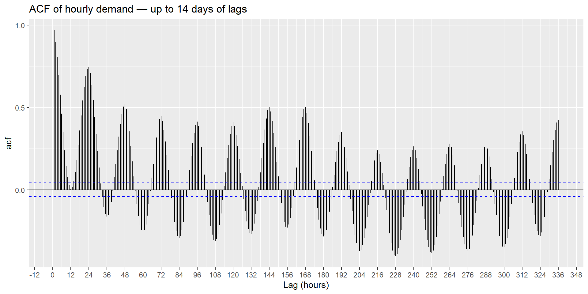
The ACF shows sharp peaks at multiples of 24 (daily cycle) and secondary peaks at multiples of 168 (weekly cycle). Both structures are strong enough to dominate the autocorrelation. A single-period ARIMA would capture at most one of them.

2.2 Train / test split

Code

vic_elec_train <- vic_elec_hourly |>
1  filter_index(~ "2014-11-30 23:00")

vic_elec_test <- vic_elec_hourly |>
  filter_index("2014-12-01 00:00" ~
2               "2014-12-14 23:00")

1: Training set: all data through November 30, 2014.
2: Test set: the first two weeks of December 2014 — 14 \times 24 = 336 hourly observations.

December in Victoria is early summer (Southern Hemisphere), meaning air conditioning load is ramping up — a genuinely challenging period to forecast and a more informative evaluation than a quiet shoulder season.

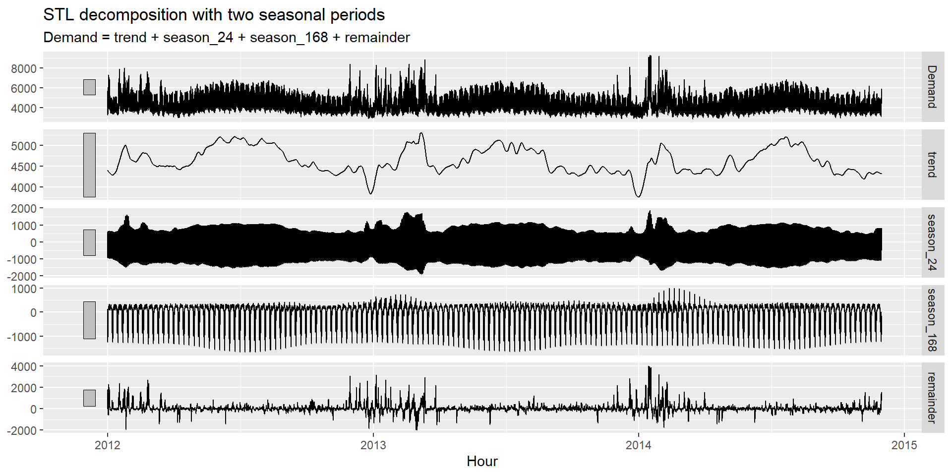
3 Approach 1 — STL with Multiple Seasonal Periods

3.1 Extending STL to multiple seasons

In Module 1, we used STL() to separate a single seasonal component from the trend-cycle. The same function supports multiple seasonal periods by stacking more than one season() call inside the formula:

Code

STL(Demand ~ season(period = 24) + season(period = 168))

Each seasonal component is estimated in sequence, holding the others fixed, until all converge. The result is one trend-cycle, one component per period, and a remainder.

3.2 Decomposition

Code

vic_elec_dcmp <- vic_elec_train |>
  model(
1    STL(Demand ~
2          season(period = 24)  +
3          season(period = 168),
        robust = TRUE)
  ) |>
  components()

vic_elec_dcmp

1: Standard STL() — the same function used in Module 1, now with two season() calls.
2: Daily seasonal component: repeating every 24 hours.
3: Weekly seasonal component: repeating every 168 hours.

Reading the decomposition

Trend: smooth multi-month movement — higher in summer (Dec–Jan) and winter (Jun–Aug) due to heating and cooling loads.
Season 24 (daily): the within-day cycle, repeating every 24 hours.
Season 168 (weekly): the within-week modulation — weekdays vs. weekends.
Remainder: what is left after extracting all components. If the model is well-specified, this should look like noise with no remaining structure.

3.3 Forecasting with `decomposition_model()`

Once we have the decomposition, we attach any univariate model to forecast the seasonally adjusted series — exactly as in Module 2:

Code

1stl_spec <- STL(Demand ~
                  season(period = 24) +
                  season(period = 168),
                robust = TRUE)

stl_fit <- vic_elec_train |>
  model(
2    STL_ETS = decomposition_model(
      stl_spec,
      ETS(season_adjust ~ season("N"))
    ),
3    STL_ARIMA = decomposition_model(
      stl_spec,
      ARIMA(season_adjust ~ PDQ(0, 0, 0))
    )
  )

1: We define the STL spec once and reuse it in both models.
2: ETS models the seasonally adjusted trend-cycle. season("N") suppresses any additional seasonal term — STL already removed both seasonal components.
3: Same structure with ARIMA. PDQ(0,0,0) suppresses seasonal ARIMA terms for the same reason.

Code

stl_fc <- stl_fit |>
  forecast(h = nrow(vic_elec_test))

4 Approach 2 — Harmonic Regression with Covariates

4.1 Why go beyond STL?

STL is a powerful univariate tool. But electricity demand has an obvious external driver that STL cannot see: temperature. On hot days, air conditioning pushes demand up. On cold days, heating does the same. The U-shaped relationship we found in Module 3.3 is real and strong.

What harmonic regression adds

Harmonic regression (Fourier terms + ARIMA errors) can incorporate external predictors alongside the seasonal patterns. STL cannot. This is the key advantage when meaningful covariates are available.

4.2 Fourier terms for multiple periods

Recall from Module 3.3 that Fourier terms approximate a seasonal pattern with K pairs of sine and cosine waves. For multiple seasonalities, we add one set per period:

y_t = \underbrace{S_{K_1}(t)}_{\text{daily, } m=24} + \underbrace{S_{K_2}(t)}_{\text{weekly, } m=168} + \beta^\top \mathbf{x}_t + \eta_t, \quad \eta_t \sim \text{ARIMA}

In fable, fourier() accepts a period argument and can be called multiple times in the same formula:

Code

ARIMA(Demand ~
        fourier(period = 24,  K = K1) +
        fourier(period = 168, K = K2) +
        PDQ(0, 0, 0))

4.2.1 Choosing K

The key parameter for each Fourier term is K — the number of sine/cosine pairs. A larger K produces a more flexible seasonal shape but adds more parameters. The standard approach is to minimize AIC_c.

Systematic K selection via grid search

The principled approach is to search over a grid of (K_1, K_2) combinations. This is computationally expensive for hourly data and is best run offline or with freeze: auto active. The code below illustrates the approach — it is not evaluated during render:

Code

expand_grid(K1 = c(6, 8, 10, 12),
            K2 = c(2, 4, 6, 8)) |>
  mutate(
    fit  = map2(K1, K2, \(k1, k2)
      vic_elec_train |>
        model(ARIMA(Demand ~
                      fourier(period = 24,  K = k1) +
                      fourier(period = 168, K = k2) +
                      PDQ(0, 0, 0),
                    stepwise = TRUE, approximation = TRUE))
    ),
    aicc = map_dbl(fit, \(m) glance(m)$AICc)
  ) |>
  select(K1, K2, aicc) |>
  arrange(aicc)

For vic_elec hourly data, K_1 = 10 and K_2 = 6 consistently perform well — they capture the main features of both seasonal patterns without overfitting. We use these values throughout.

4.3 Adding temperature and WorkDay

Following FPP3, we model temperature with a piecewise linear function: a linear term plus a hockey-stick that activates above 18°C:

\text{Temp effect} = \beta_1 T_t + \beta_2 \max(T_t - 18,\; 0)

The intuition: below 18°C, demand increases as temperature falls (heating load). Above 18°C, demand increases as temperature rises (cooling load). The slope changes at the knot at 18°C.

Code

fourier_fit <- vic_elec_train |>
  model(
1    fourier_only = ARIMA(
      Demand ~
        fourier(period = 24,  K = 10) +
        fourier(period = 168, K = 6)  +
        PDQ(0, 0, 0),
      stepwise = TRUE, approximation = TRUE
    ),
2    fourier_cov = ARIMA(
      Demand ~
        fourier(period = 24,  K = 10) +
        fourier(period = 168, K = 6)  +
        Temperature +
3        I(pmax(Temperature - 18, 0)) +
4        WorkDay +
        PDQ(0, 0, 0),
      stepwise = TRUE, approximation = TRUE
    )
  )

1: Baseline harmonic model — Fourier terms only, no external predictors.
2: Full model: Fourier terms + piecewise temperature + WorkDay indicator.
3: pmax(Temperature - 18, 0) equals zero below 18°C and T - 18 above — the hockey-stick knot. I() protects the arithmetic inside the formula.
4: WorkDay captures the weekday demand premium beyond what the weekly Fourier terms already model.

Why a knot at 18°C?

18°C is a typical thermal comfort threshold for Melbourne’s climate — roughly the temperature above which mechanical cooling becomes widespread. FPP3 uses this same knot. It has a clear physical interpretation and works well empirically.

4.4 The temperature forecasting problem

Adding temperature as a predictor immediately raises the challenge we faced in Module 3.3: to forecast demand, we need future temperature values.

If we use observed future temperatures (ex-post), the model looks better than it would in real deployment.
If we use a meteorological forecast, we inherit all the uncertainty from that forecast.
Temperature is hard to forecast reliably beyond a few days ahead — and errors compound.

Residuals still contain temperature information

Even with the piecewise linear temperature term, residuals of fourier_cov will show some remaining pattern linked to temperature extremes — particularly during heatwaves. The linear + hockey-stick approximation captures the average relationship but misses nonlinear tail behavior during extreme events.

This is a known limitation acknowledged in FPP3: electricity demand models with temperature covariates rarely achieve white-noise residuals. The residuals still carry information we have not fully captured.

For the forecast we use a scenario approach — constant temperature at 25°C (a mild early-summer day in Victoria):

Code

vic_elec_future <- new_data(vic_elec_train, nrow(vic_elec_test)) |>
  mutate(
1    Temperature = 25,
2    Holiday     = FALSE,
    WorkDay     = wday(Hour) %in% 2:6
  )

1: Conservative scenario: constant 25°C throughout the two-week horizon.
2: No public holidays in the first two weeks of December in Victoria.

Code

fourier_fc <- fourier_fit |>
  forecast(new_data = vic_elec_future)

5 Model Comparison

5.1 Accuracy

Code

bind_rows(stl_fc, fourier_fc) |>
  accuracy(vic_elec_hourly) |>
  select(.model, RMSE, MAE, MAPE, MASE) |>
  arrange(RMSE)

5.2 Residual diagnostics

Code

stl_fit |>
  select(STL_ETS) |>
  gg_tsresiduals(lag_max = 48)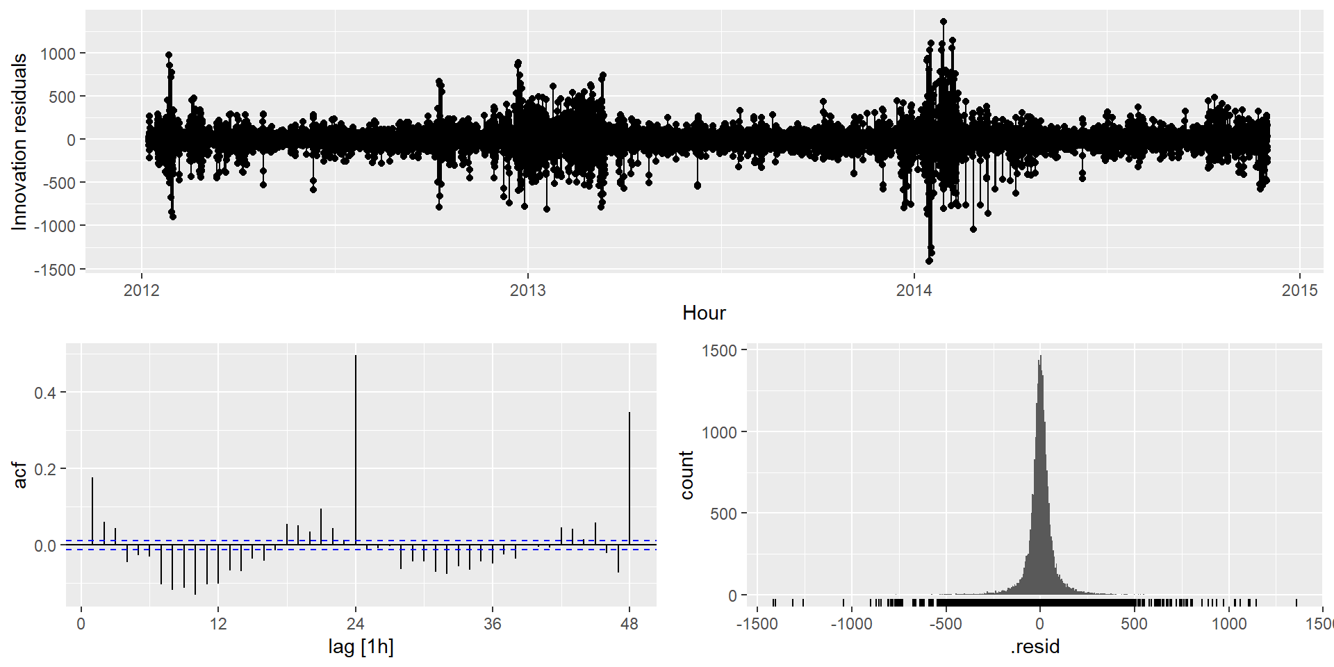

Code

stl_fit |>
  select(STL_ARIMA) |>
  gg_tsresiduals(lag_max = 48)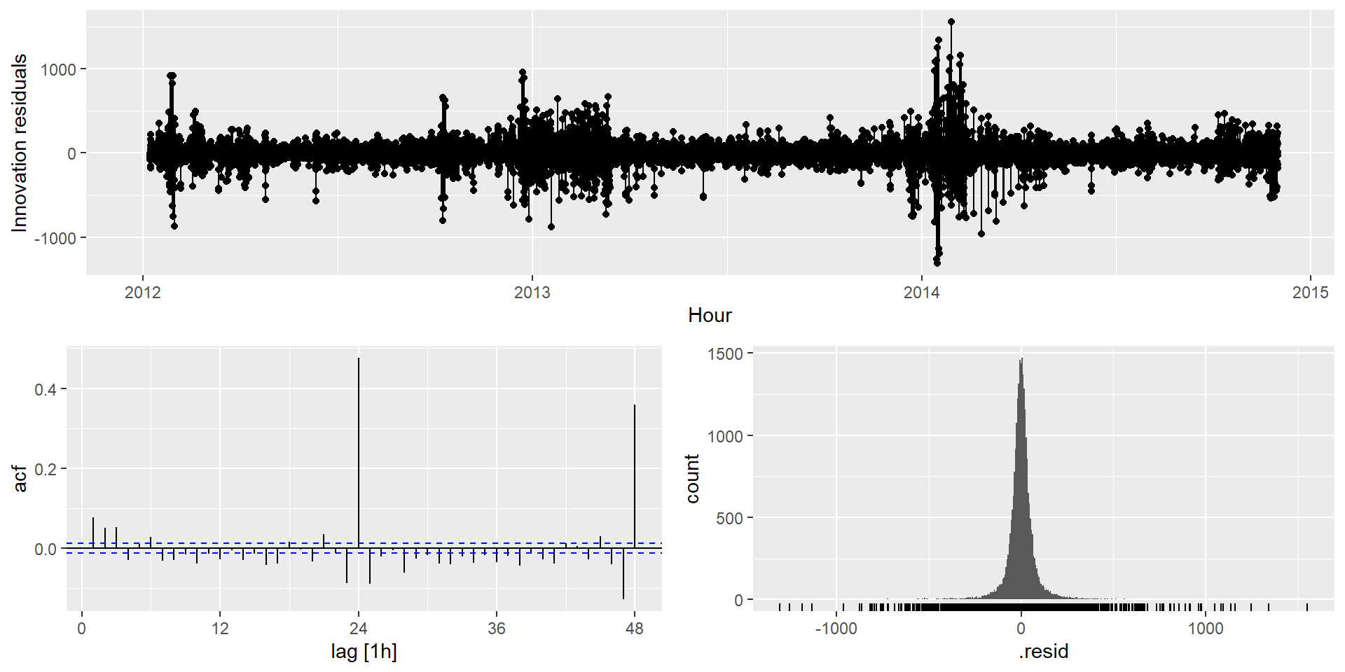

Code

fourier_fit |>
  select(fourier_cov) |>
  gg_tsresiduals(lag_max = 48)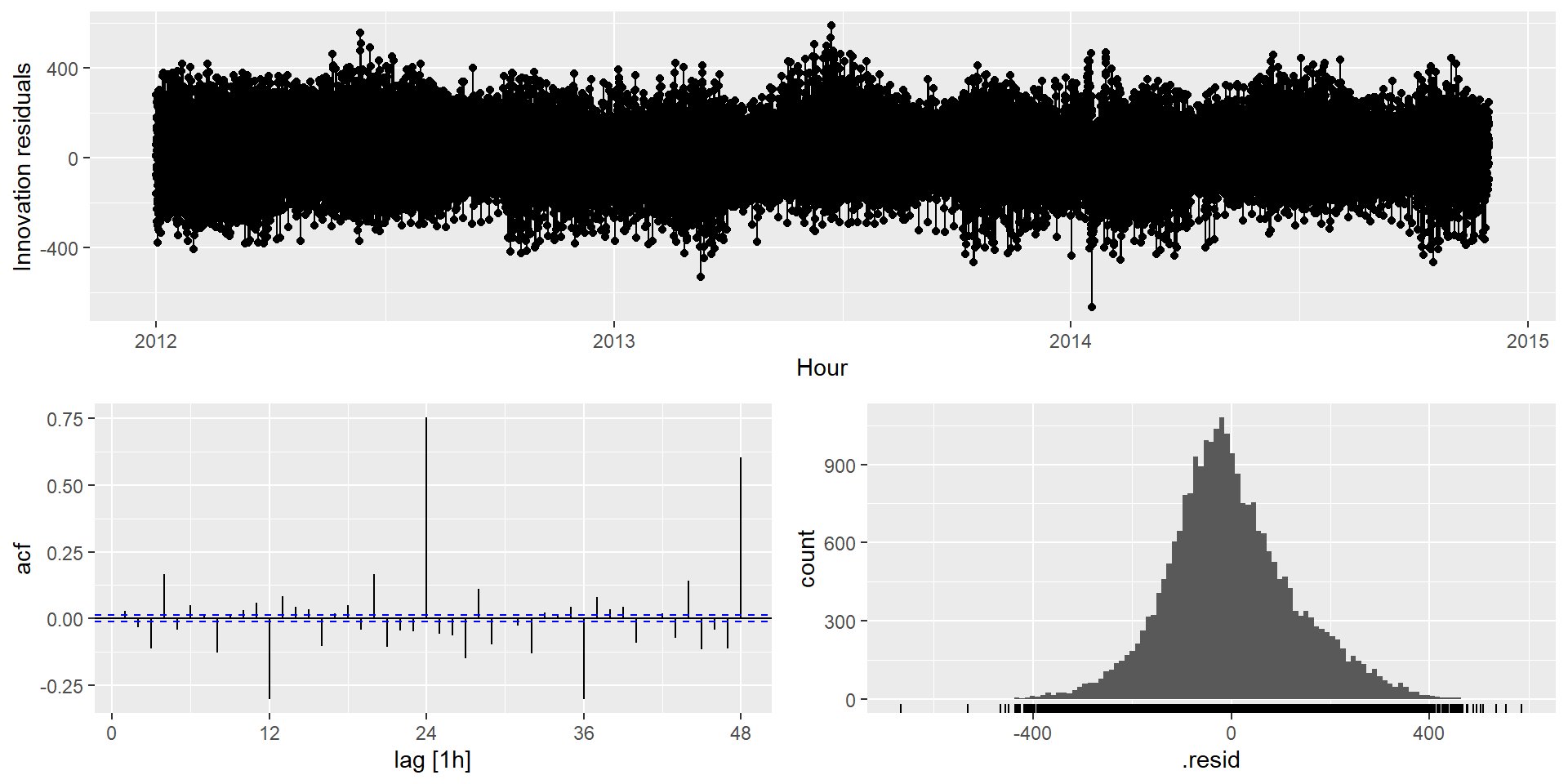

5.3 When to use each approach

Decision guide

Situation	Recommended approach
No external predictors available	STL — clean, fast, interpretable decomposition
External predictors available and forecastable	Fourier + covariates — captures more signal
Predictors hard to forecast (e.g., spot temperatures)	STL or Fourier-only — avoid inheriting predictor uncertainty
Need interpretable components for stakeholders	STL — the decomposition plot is self-explanatory
Complex, irregular seasonality with holiday effects	Consider Prophet (Module 3.4)

What about TBATS?

FPP3 mentions TBATS (Trigonometric seasonality, Box-Cox transformation, ARMA errors, Trend, Seasonal components) as another approach for complex seasonality. TBATS handles multiple seasonal periods and non-integer periods automatically.

However, TBATS is implemented in the older forecast package (forecast::tbats()), not in fable. Since we work exclusively within the fable / tidyverts ecosystem, we do not cover it in this course. The STL + Fourier combination achieves comparable results with a more transparent and modular workflow.

Curious? See ?forecast::tbats and FPP3 §12.1 for details.

6 In-Class Exercise: Call Centre Demand

6.1 The dataset

The bank_calls dataset records the number of calls arriving at a North American commercial bank call centre, measured at 5-minute intervals over 33 weeks. This is a classic complex seasonality dataset with within-day and within-week structure — and an important twist: the call centre is closed overnight and on weekends.

Code

bank_calls

6.2 Exercise 1 — Exploratory Analysis

Exercise 1

Begin by exploring bank_calls visually.

a) Use the plot above — zoom in on a single week and describe what you see in terms of daily and weekly patterns.

b) Create seasonal plots using gg_season() for the daily and weekly periods. What are the dominant features of each?

c) Plot the ACF up to at least 7 days of lags. At which lags do you see the strongest spikes?

Hint — Seasonal periods

At 5-minute intervals, one day has 12 \times 24 = 288 observations and one week has 288 \times 7 = 2{,}016 observations. Both should be visible in the ACF.

Note that the call centre is closed overnight and on weekends — this creates blocks of zeros that will dominate the decomposition if not handled carefully.

6.3 Exercise 2 — Data Preparation

Exercise 2

The 5-minute granularity is too fine for practical modeling.

a) Aggregate bank_calls to half-hourly frequency using index_by() and summarise(). Use sum() for calls.

b) Handle the overnight and weekend gaps. Are they true zeros (call centre closed) or missing values? Use fill_gaps() if needed and decide how to treat them in the model.

c) Create a train/test split reserving the last 2 weeks as the test set.

Hint — Handling gaps

bank_calls has implicit gaps for overnight hours and weekends. Use fill_gaps(Calls = 0) before aggregating to make them explicit. Think carefully about whether your model should learn from these zeros or whether filtering them out makes more sense.

6.4 Exercise 3 — Model Fitting

Exercise 3

Fit at least two models to your training data:

a) An STL-based model with two season() calls for the daily and weekly periods. Use either ETS or ARIMA for the seasonally adjusted component.

b) A harmonic regression model (Fourier terms + ARIMA errors) with both periods. Start with K_1 = 6 for the daily period and K_2 = 3 for the weekly period, adjusting by AIC_c if you want to explore further.

c) Inspect residuals from both models using gg_tsresiduals(). Is there remaining autocorrelation? What does the ACF look like around lags 48 and 336?

Hint — Fourier K for half-hourly data

For half-hourly data, the daily period is m_1 = 48 and the weekly period is m_2 = 336. Start with small K values and use stepwise = TRUE, approximation = TRUE inside ARIMA() — exact search over periods this large is very slow.

6.5 Exercise 4 — Forecast Evaluation

Exercise 4

a) Generate 2-week-ahead forecasts from both models and compute accuracy metrics on the test set. Which model performs better?

b) Plot the forecasts overlaid on the test set. Does the model correctly capture the overnight shutdown and weekend pattern? What happens if it does not?

c) Reflection: bank_calls has no obvious external covariate like temperature. Does that make STL the natural choice here, or can you think of predictors that might be useful in a real deployment?

Hint — Non-zero overnight forecasts

If your model produces non-zero forecasts during overnight and weekend hours, it does not know the call centre is closed. Consider adding an IsOpen binary indicator as a predictor, or filter out closed hours before modeling and evaluate only on open hours.

7 Summary

7.1

When a series has multiple seasonal periods, standard STL, ETS, and ARIMA models are not sufficient — they can handle at most one seasonal cycle cleanly.
STL with multiple season() calls extends the decomposition to an arbitrary number of periods, each estimated in sequence. Forecasting uses decomposition_model() with any univariate model for the seasonally adjusted series.
Harmonic regression (Fourier terms + ARIMA errors) handles multiple periods by including one set of Fourier terms per period in the formula. Its key advantage: external predictors can be added directly alongside the Fourier terms — something STL cannot do.
For electricity demand, temperature enters as a piecewise linear function with a knot at 18°C. Residuals may still carry temperature-linked structure near extremes — a known limitation of linear covariate approximations in demand modeling.
Choosing K for each Fourier period is done by AIC_c comparison. For long seasonal periods, use stepwise = TRUE, approximation = TRUE inside ARIMA() to keep computation manageable.

The Module 4 picture so far

Session	What we added	Key tool
4.1 (now)	Multiple seasonal periods	STL + multiple seasons, Fourier terms
4.2	Robustness and forecast combinations	Bootstrapping, bagging
4.3	Robust evaluation	Time series cross-validation
4.4	Hierarchical structure	Reconciliation

1 The Data

1.1 From half-hourly to hourly

1.2 Exploratory analysis

2 Identifying Multiple Seasonality

2.1 Seasonal plots

2.2 Train / test split

3 Approach 1 — STL with Multiple Seasonal Periods

3.1 Extending STL to multiple seasons

3.2 Decomposition

3.3 Forecasting with decomposition_model()

4 Approach 2 — Harmonic Regression with Covariates

4.1 Why go beyond STL?

4.2 Fourier terms for multiple periods

4.2.1 Choosing K

4.3 Adding temperature and WorkDay

4.4 The temperature forecasting problem

5 Model Comparison

5.1 Accuracy

5.2 Residual diagnostics

5.3 When to use each approach

6 In-Class Exercise: Call Centre Demand

6.1 The dataset

6.2 Exercise 1 — Exploratory Analysis

6.3 Exercise 2 — Data Preparation

6.4 Exercise 3 — Model Fitting

6.5 Exercise 4 — Forecast Evaluation

7 Summary

7.1

3.3 Forecasting with `decomposition_model()`