Dynamic & Harmonic Regression

Modified

May 8, 2026

Code

1library(plotly)

1: In addition to the regular packages, here we’ll use plotly for interactive plots.

In the previous session, we built a multiple regression model for US consumption:

y_{t,\text{Cons.}} = \beta_0 + \beta_1 x_{t,\text{Inc.}} + \beta_2 x_{t,\text{Prod.}} + \beta_3 x_{t,\text{Sav.}} + \beta_4 x_{t,\text{Unemp.}} + \varepsilon_t

The model improved substantially over the simple version — \bar{R}^2 went from ~0.15 to ~0.75, and the residuals looked much closer to white noise.

But “much closer” is not the same as “white noise.” Let’s check:

Code

us_change_fit_mult |>
  augment() |>
  features(.resid, ljung_box, lag = 10, dof = 5)

The p-value is not zero, but in practice with real data there is nearly always some residual autocorrelation left after TSLM. And that matters:

What autocorrelated residuals cost us

If \varepsilon_t is autocorrelated, OLS is still unbiased — but standard errors are wrong, confidence intervals are wrong, and prediction intervals are wrong. The model is leaving structure on the table that could be captured.

The culprit is the white noise assumption on \varepsilon_t:

\varepsilon_t \overset{\text{iid}}{\sim} N(0, \sigma^2)

What if instead of forcing this, we modeled whatever autocorrelation remains?

The upgrade: relax the white noise assumption

Model	Error term
TSLM	\varepsilon_t \overset{\text{iid}}{\sim} N(0,\sigma^2) — must be white noise
Dynamic regression	\eta_t \sim \text{ARIMA}(p,d,q) — can be autocorrelated

Same predictors. Same regression structure. One assumption relaxed.

1 Dynamic Regression

1.1 The Model

The dynamic regression model replaces the white noise error \varepsilon_t with \eta_t, which is allowed to follow an ARIMA process:

y_t = \beta_0 + \beta_1 x_{1,t} + \cdots + \beta_k x_{k,t} + \eta_t

\eta_t \sim \text{ARIMA}(p, d, q)(P, D, Q)_m

The model still has white noise — it just lives one level deeper. There are now two distinct error terms:

Two error terms

\eta_t — the regression error: how far y_t is from the regression surface. Still autocorrelated, now modeled explicitly.
\varepsilon_t — the ARIMA innovation: the white noise that drives \eta_t. This is the only truly random component.

We diagnose the model using \hat{\varepsilon}_t, not \hat{\eta}_t.

1.1.1 Stationarity: Models in Levels vs. in Differences

All variables must be stationary

Dynamic regression requires that both y_t and all predictors x_{k,t} are stationary. Check each variable with unit root tests before fitting.

When differencing is needed, there are two natural cases:

Model in levels — no variable requires differencing. The regression is fitted directly on the original (or transformed) series. This is the most common case when all variables are already stationary, as in us_change.
Model in differences — one or more variables need differencing to achieve stationarity. In this case, all variables are differenced simultaneously to keep the model internally consistent. Specifying pdq(d = 1) in ARIMA() does this automatically.

Stochastic vs. deterministic trends

A closely related question is whether a trend in the data is deterministic (captured by a trend() term in TSLM — predictable, fixed slope) or stochastic (captured by differencing in ARIMA — the trend wanders randomly over time). In practice, stochastic trends are far more common in economic and business data. See FPP3 §10.1 for a detailed comparison with forecasting implications.

1.1.2 Fitting in R

ARIMA() handles dynamic regression by simply adding predictors to the right-hand side of the formula — the same syntax as TSLM():

Code

# TSLM — white noise errors assumed
TSLM(y ~ x1 + x2)

# Dynamic regression — ARIMA errors, order chosen automatically
ARIMA(y ~ x1 + x2)

# Model in differences: force differencing on all variables
ARIMA(y ~ x1 + x2 + pdq(d = 1))

1.2 Example: US Consumption

1.2.1 Fitting the Dynamic Regression

Code

us_change_fit_dyn <- us_change |>
  model(
1    tslm    = TSLM(Consumption ~ Income + Production +
                     Savings + Unemployment),
2    dynamic = ARIMA(Consumption ~ Income + Production +
                      Savings + Unemployment)
  )

us_change_fit_dyn |>
  select(dynamic) |>
  report()

1: Our previous model — kept here for direct comparison.
2: Same predictors, same formula structure. ARIMA() selects the error order automatically via AIC_c.

Series: Consumption 
Model: LM w/ ARIMA(0,1,2) errors 

Coefficients:
          ma1     ma2  Income  Production  Savings  Unemployment
      -1.0882  0.1118  0.7472      0.0370  -0.0531       -0.2096
s.e.   0.0692  0.0676  0.0403      0.0229   0.0029        0.0986

sigma^2 estimated as 0.09588:  log likelihood=-47.13
AIC=108.27   AICc=108.86   BIC=131.25

1.2.2 Two Types of Residuals

We can extract both error types from the fitted model:

Code

bind_rows(
1  `Regression errors` = as_tibble(
    residuals(us_change_fit_dyn |> select(dynamic),
              type = "regression")),
2  `ARIMA innovations` = as_tibble(
    residuals(us_change_fit_dyn |> select(dynamic),
              type = "innovation")),
  .id = "type"
) |>
  ggplot(aes(x = Quarter, y = .resid)) +
  geom_line() +
  facet_wrap(~ type, nrow = 2, scales = "free_y") +
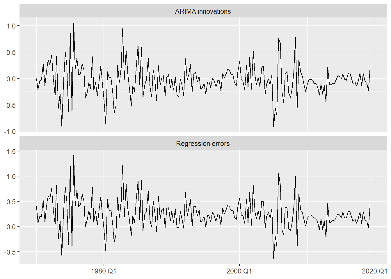
  labs(y = NULL, x = NULL)

1: type = "regression" → \hat{\eta}_t: the regression residuals. These still have autocorrelation structure, now captured by the ARIMA component.
2: type = "innovation" → \hat{\varepsilon}_t: what should be white noise. This is what we diagnose.

1.2.3 Residual Diagnostics

Code

us_change_fit_dyn |>
  select(dynamic) |>
  gg_tsresiduals()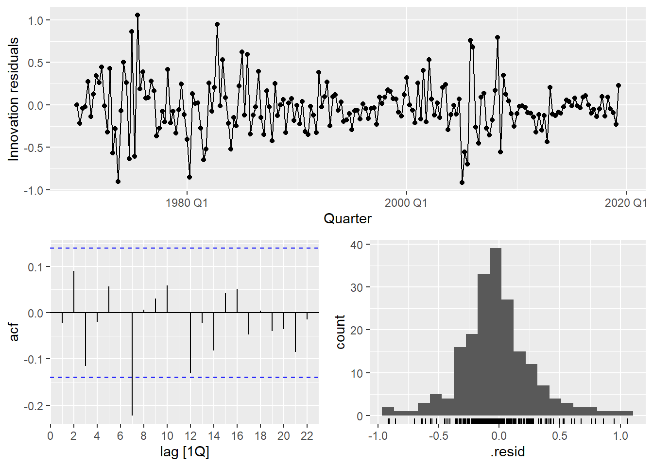

Code

us_change_fit_dyn |>
  select(dynamic) |>
  augment() |>
  features(.innov, ljung_box,
           lag = 10,
1           dof = us_change_fit_dyn |>
                   select(dynamic) |>
                   coefficients() |>
                   filter(str_detect(term, "^ar|^ma")) |>
                   nrow())

1: dof is computed dynamically as the number of estimated AR and MA coefficients — always matches the fitted model regardless of order selected.

1.2.4 Does It Actually Improve Things?

Let’s compare the two models side by side on a held-out test set:

Code

us_change_train <- us_change |> filter_index(. ~ "2015 Q4")
us_change_test  <- us_change |> filter_index("2016 Q1" ~ .)

us_change_fit_cv <- us_change_train |>
  model(
    tslm    = TSLM(Consumption ~ Income + Production + Savings + Unemployment),
    dynamic = ARIMA(Consumption ~ Income + Production + Savings + Unemployment)
  )

us_change_fit_cv |>
  forecast(new_data = us_change_test) |>
  accuracy(us_change_test) |>
  select(.model, RMSE, MAE, MAPE)

Key insight

The dynamic regression model passes the Ljung-Box test — something the TSLM could not. By modeling the residual autocorrelation explicitly with ARIMA, we get valid standard errors, correct prediction intervals, and typically better out-of-sample accuracy.

1.3 Forecasting

Forecasting works exactly as in Session 3.2 — you still need future values of the predictors, and the same three strategies apply (ex-ante, ex-post, scenario-based).

The only practical difference: you use new_data() to build the future dataset and pass it to forecast(). The ARIMA component of the errors is projected forward automatically.

1.3.1 Scenario Forecast

Code

us_change_future <- us_change |>
1  pivot_longer(-c(Quarter, Consumption),
               names_to = "variable") |>
2  model(MEAN(value)) |>
3  forecast(h = 8) |>
  as_tsibble() |>
  select(-c(.model, value)) |>
4  pivot_wider(names_from  = variable,
              values_from = .mean)

us_change_fit_dyn |>
  select(dynamic) |>
  forecast(new_data = us_change_future) |>
  autoplot(tail(us_change, 60)) +
  labs(
    title    = "US Consumption: dynamic regression forecast",
    subtitle = "Baseline scenario: predictors forecast with MEAN",
    y = "% change", x = NULL
  )

1: Pivot the four predictor columns to long format — each variable becomes its own series, identified by variable.
2: A single model() call fits MEAN to each predictor simultaneously.
3: A single forecast() produces 8-step-ahead forecasts for all predictors at once.
4: Pivot back to wide format so each predictor has its own column, matching the structure that forecast() expects in new_data.

Swapping the forecast method

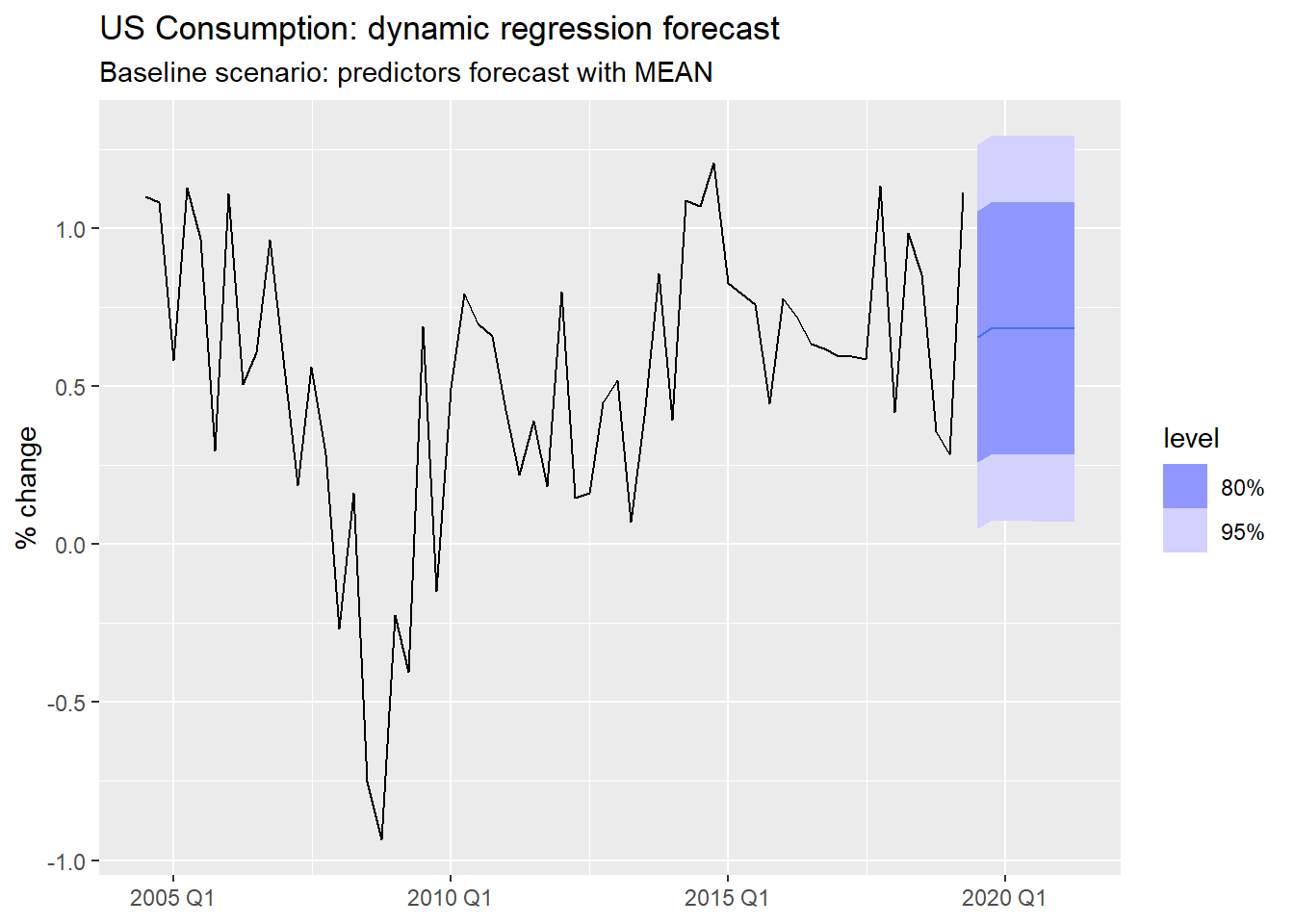
Because the predictors go through a proper model() |> forecast() pipeline, changing the scenario is a one-word edit:

Code

model(MEAN(value))          # flat forecast at the historical mean
model(NAIVE(value))         # last observed value carried forward
model(RW(value ~ drift()))  # linear extrapolation of the recent trend
model(ARIMA(value))         # best ARIMA for each predictor

MEAN is appropriate here because all us_change variables are stationary percentage changes — the historical mean is a reasonable “neutral” projection. For predictors with trend, RW(drift) or ARIMA would be more honest.

1.3.2 TSLM vs. Dynamic: Prediction Intervals

Code

us_change_fit_dyn |>
  forecast(new_data = us_change_future) |>
1  autoplot(tail(us_change, 60), level = 80, alpha = 0.6) +
  labs(
    title = "Modeling ARIMA errors narrows prediction intervals",
    subtitle = "80% prediction intervals shown",
    y = "% change", x = NULL
  )

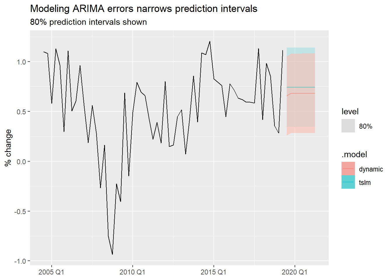
1: Both models are overlaid on the same axes. The difference in interval width is immediately visible.

The prediction interval caveat

Dynamic regression intervals assume future predictor values are known exactly. When they are estimated (as in the scenario above), true uncertainty is larger than what the intervals show. This applies equally to TSLM — dynamic regression does not make this problem worse, it just fixes the autocorrelation problem.

1.4 Example: Electricity Demand

The us_change example was clean: stationary series, linear relationship. Electricity demand pushes two things further:

A nonlinear relationship between the predictor and the response
A categorical predictor (day type) alongside a continuous one

1.4.1 The Data

Daily electricity demand in Victoria, Australia (2014):

Two patterns are immediately clear:

U-shaped (quadratic) relationship with temperature — both very hot and very cold days increase demand.
Day type matters: weekdays > weekends > holidays.

This gives us the model:

y_t = \beta_0 + \beta_1 T_t + \beta_2 T_t^2 + \beta_3 D_{\text{day type}} + \eta_t, \quad \eta_t \sim \text{ARIMA}

1.4.2 Fitting the Model

Code

vic_elec_fit <- vic_elec_daily |>
  model(
1    dynamic = ARIMA(Demand ~ Temperature + I(Temperature^2) +
2            (Day_Type == "Weekday"))
  )

report(vic_elec_fit)

1: I(Temperature^2) adds the quadratic term. The I() wrapper is required to protect arithmetic inside the formula.
2: A logical expression that becomes a binary indicator: TRUE (1) for weekdays, FALSE (0) otherwise.

Series: Demand 
Model: LM w/ ARIMA(2,1,2)(2,0,0)[7] errors 

Coefficients:
          ar1     ar2      ma1      ma2    sar1    sar2  Temperature
      -0.1093  0.7226  -0.0182  -0.9381  0.1958  0.4175      -7.6135
s.e.   0.0779  0.0739   0.0494   0.0493  0.0525  0.0570       0.4482
      I(Temperature^2)  Day_Type == "Weekday"TRUE
                0.1810                    30.4040
s.e.            0.0085                     1.3254

sigma^2 estimated as 44.91:  log likelihood=-1206.11
AIC=2432.21   AICc=2432.84   BIC=2471.18

How many day-type categories?

The choice of how to encode day type depends on the question you want to answer:

Binary — Day_Type == "Weekday": distinguishes working days from non-working days (weekends + holidays collapsed together). Simpler, fewer parameters, often sufficient.
Two dummies — Day_Type == "Weekday" and Day_Type == "Weekend" (holidays as baseline): allows weekends and holidays to have different demand profiles. Useful if your data shows a meaningful difference between the two.

Neither is universally better — let residual diagnostics and AIC_c guide the choice.

1.4.3 Diagnostics & Scenario Forecast

Code

vic_elec_fit |> gg_tsresiduals()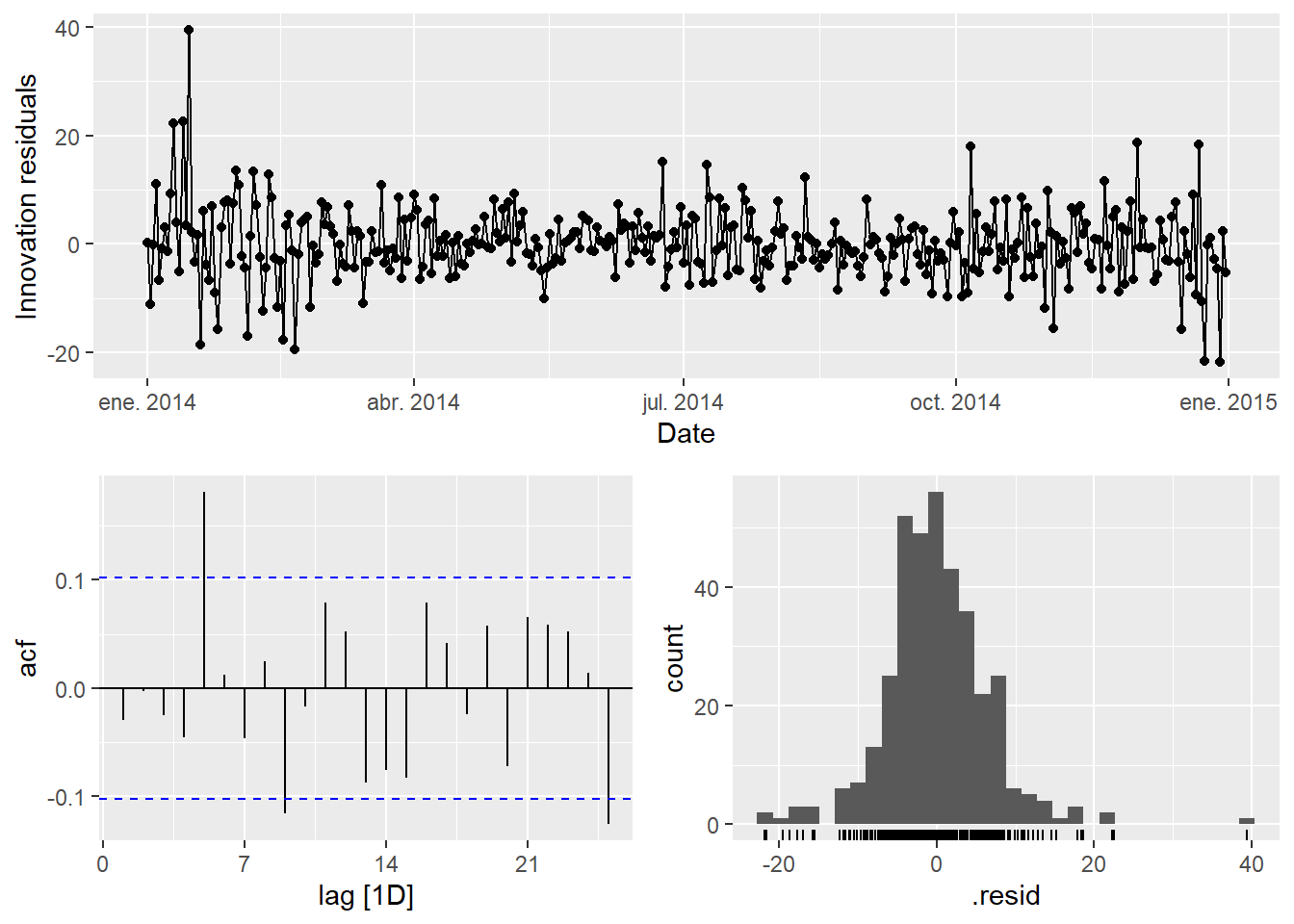

Code

vic_elec_fit |>
  augment() |>
  features(.innov, ljung_box, dof = 8, lag = 14)

Heteroscedastic residuals

Variance is higher during January–February (Australian summer peak). Point estimates remain valid, but prediction intervals may be too narrow for extreme temperature periods.

Code

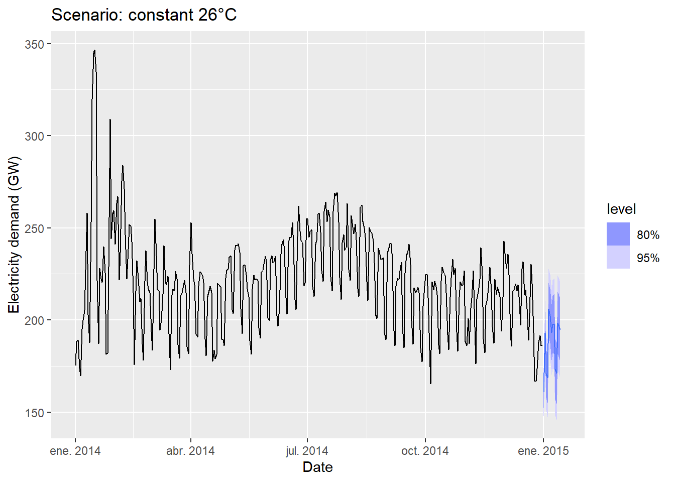
vic_elec_future_26 <- new_data(vic_elec_daily, 14) |>
  mutate(
    Temperature = 26,
    Holiday     = c(TRUE, rep(FALSE, 13)),
    Day_Type    = case_when(
      Holiday              ~ "Holiday",
      wday(Date) %in% 2:6  ~ "Weekday",
      TRUE                 ~ "Weekend"
    )
  )

Code

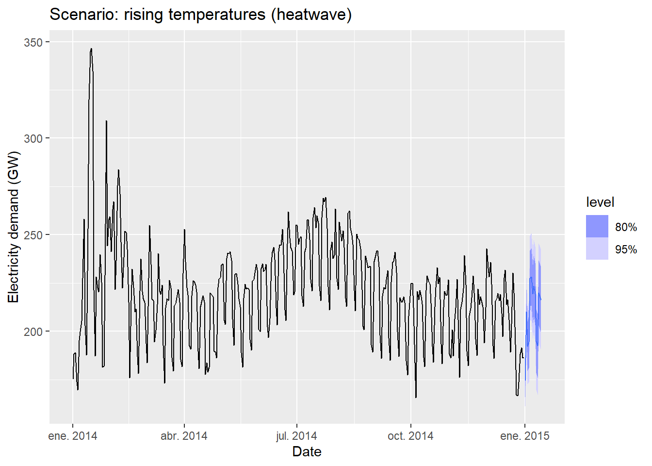
vic_elec_future_hw <- new_data(vic_elec_daily, 14) |>
  mutate(
1    Temperature = c(seq(31, 34), 33, rep(34, 3), rep(33, 6)),
    Holiday     = c(TRUE, rep(FALSE, 13)),
    Day_Type    = case_when(
      Holiday              ~ "Holiday",
      wday(Date) %in% 2:6  ~ "Weekday",
      TRUE                 ~ "Weekend"
    )
  )

1: A realistic meteorological forecast — considerably hotter than 26°C.

1.5 Lagged Predictors

So far we have assumed that the predictor x_t affects y_t at the same point in time. But many real-world relationships have a delay: the cause happens now, the effect shows up later.

Advertising spend in month t drives sales in months t, t+1, t+2, … as the message reaches new customers gradually.
Interest rate changes take months to affect housing starts or consumer credit.
Rainfall in January affects agricultural output in March or April.
Hiring a new employee today affects productivity in weeks t+4, t+5, … after onboarding.

Models that include x_t at multiple lags are called distributed lag models:

y_t = \beta_0 + \delta_0 x_t + \delta_1 x_{t-1} + \delta_2 x_{t-2} + \cdots + \delta_k x_{t-k} + \eta_t

Each \delta_j captures the effect of x that occurs j periods after the predictor.

1.5.1 Example: Advertising and Sales

The fpp3 package includes the insurance dataset: monthly US insurance quotes (a proxy for sales) and TV advertising expenditure:

1.5.2 Fitting Distributed Lag Models

We fit four models with increasing lag depth to find how long the advertising effect persists:

Code

insurance_fit <- insurance |>
  model(
1    lag0 = ARIMA(Quotes ~ pdq(d = 0) +
                   TVadverts),
    lag1 = ARIMA(Quotes ~ pdq(d = 0) +
2                   TVadverts + lag(TVadverts)),
    lag2 = ARIMA(Quotes ~ pdq(d = 0) +
                   TVadverts + lag(TVadverts) +
3                   lag(TVadverts, 2)),
    lag3 = ARIMA(Quotes ~ pdq(d = 0) +
                   TVadverts + lag(TVadverts) +
                   lag(TVadverts, 2) + lag(TVadverts, 3))
  )

glance(insurance_fit) |>
  select(.model, AICc) |>
  arrange(AICc)

1: pdq(d = 0) fixes the differencing order to zero — both series are stationary.
2: lag(TVadverts) is x_{t-1}: advertising from the previous month.
3: lag(TVadverts, 2) is x_{t-2}: advertising from two months ago.

1.5.3 Best Model & Interpretation

Code

insurance_fit |>
  select(lag1) |>
  report()

Series: Quotes 
Model: LM w/ ARIMA(1,0,2) errors 

Coefficients:
         ar1     ma1     ma2  TVadverts  lag(TVadverts)  intercept
      0.5123  0.9169  0.4591     1.2527          0.1464     2.1554
s.e.  0.1849  0.2051  0.1895     0.0588          0.0531     0.8595

sigma^2 estimated as 0.2166:  log likelihood=-23.94
AIC=61.88   AICc=65.38   BIC=73.7

Reading the lag coefficients

The coefficient on TVadverts (\delta_0) is the immediate effect: one unit increase in advertising this month increases quotes by \delta_0 units this month.

The coefficient on lag(TVadverts) (\delta_1) is the one-period carry-over: the additional effect that arrives one month later.

Together, the total effect of a sustained 1-unit increase in advertising is \delta_0 + \delta_1 + \cdots — the sum of all lag coefficients.

1.5.4 Forecasting with Lagged Predictors

When forecasting, you need future values of x_t and the most recent observed values of x to fill in the lags:

Code

insurance_future <- new_data(insurance, 20) |>
1  mutate(TVadverts = 8)

insurance_fit |>
  select(lag1) |>
  forecast(new_data = insurance_future) |>
  autoplot(insurance) +
  labs(title = "Insurance quotes forecast: lag-1 distributed lag model",
       subtitle = "Scenario: advertising held constant at 8",
       y = "Quotes (thousands)", x = NULL)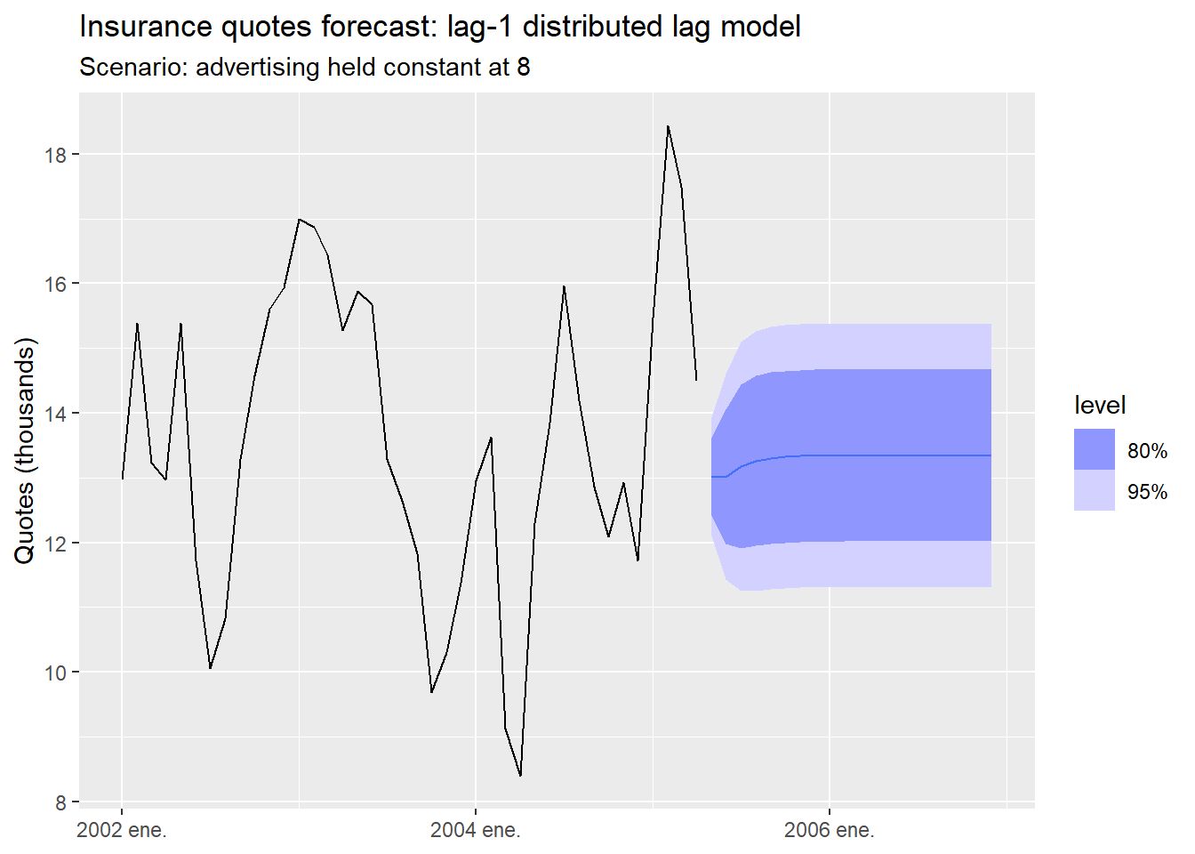

1: We assume a constant advertising level of 8 for the forecast horizon — a simple scenario.

When to use lagged predictors vs. current predictors

Situation	Prefer
Effect is immediate (prices, temperature)	Current x_t
Effect has a known delay (advertising, policy)	x_t + lags
Delay length is unknown	Fit models with 0, 1, 2, … lags and compare with AIC_c
Predictor is hard to forecast	Lags are known at forecast time — a practical advantage

The last point is important: if x_t is hard to forecast, using x_{t-k} instead means the predictor is already observed when you need to make the forecast. Lags can turn an ex-ante problem into an ex-post one.

2 Harmonic Regression

2.1 When Seasonal Dummies Aren’t Enough

The electricity demand example above used daily data. Demand has an obvious annual seasonal pattern (m = 365). If we wanted to capture it with dummy variables, we would need 364 of them.

That is impractical. The same problem appears with:

Data frequency	Seasonal period
Daily (annual cycle)	m = 365
Weekly	m = 52
Half-hourly (daily cycle)	m = 48

Recall from Session 3.2

We first saw Fourier terms mentioned as a footnote in regression.qmd — they were promised as the solution for large m. This is where we deliver on that promise.

2.1.1 Fourier Terms

Any periodic pattern can be approximated by a sum of sine and cosine waves:

S_K(t) = \sum_{k=1}^{K} \left[ a_k \cos\!\left(\frac{2\pi k t}{m}\right) + b_k \sin\!\left(\frac{2\pi k t}{m}\right) \right]

m — seasonal period
K — number of Fourier pairs (controls flexibility)

The key parameter: K

Small K → smooth, slowly-varying seasonal pattern
Large K → complex, flexible seasonal pattern (but more parameters)
K = m/2 → identical to using m - 1 seasonal dummies

Choose K by minimizing AIC_c.

2.1.2 Advantages and Limitations

Advantages over seasonal dummies:

Works for any m, no matter how large
Handles multiple seasonalities simultaneously
Smooth patterns with small K → fewer parameters
Short-run dynamics handled by ARIMA errors

Limitations:

Seasonal pattern assumed fixed over time
Requires choosing K
Less intuitive than dummies for small m

2.2 Example: Australian Café Spending

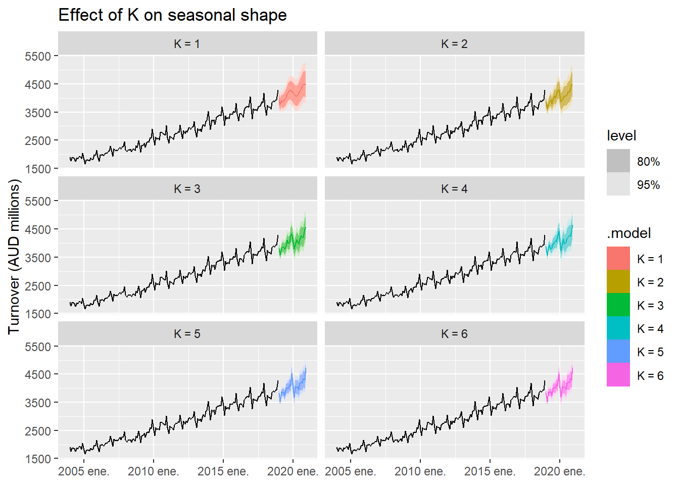
Monthly retail turnover for cafés and restaurants in Australia (2004–2018). A clean example of a monthly series with strong, stable seasonality — ideal for comparing values of K:

Code

aus_cafe <- aus_retail |>
  filter(
    Industry == "Cafes, restaurants and takeaway food services",
    year(Month) %in% 2004:2018
  ) |>
  summarise(Turnover = sum(Turnover))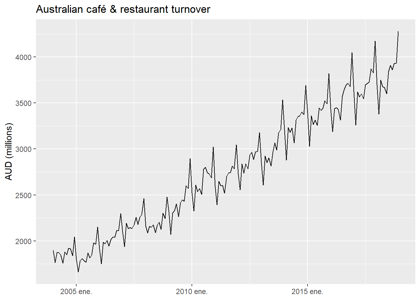

2.2.1 Fitting Multiple Values of K

Code

cafe_fit <- aus_cafe |>
  model(
1    `K = 1` = ARIMA(log(Turnover) ~ fourier(K = 1) + PDQ(0, 0, 0)),
    `K = 2` = ARIMA(log(Turnover) ~ fourier(K = 2) + PDQ(0, 0, 0)),
    `K = 3` = ARIMA(log(Turnover) ~ fourier(K = 3) + PDQ(0, 0, 0)),
    `K = 4` = ARIMA(log(Turnover) ~ fourier(K = 4) + PDQ(0, 0, 0)),
    `K = 5` = ARIMA(log(Turnover) ~ fourier(K = 5) + PDQ(0, 0, 0)),
2    `K = 6` = ARIMA(log(Turnover) ~ fourier(K = 6) + PDQ(0, 0, 0))
  )

glance(cafe_fit) |>
  select(.model, AICc, BIC) |>
  arrange(AICc)

1: PDQ(0,0,0) suppresses seasonal ARIMA terms — Fourier handles the seasonality entirely.
2: For monthly data (m = 12), K = 6 is exactly equivalent to using 11 seasonal dummies.

2.2.2 Comparing Forecasts Across K

What to look for

K = 1–2: Very smooth, nearly sinusoidal — misses the multi-peak retail calendar
K = 3–4: Usually the AIC_c winner; captures the main features of Australian retail seasonality
K = 6: Reproduces seasonal dummies exactly — can overfit the historical pattern

2.3 What Comes Next?

The café example had one seasonal period (m = 12, monthly). But what if a series has more than one?

Consider electricity demand measured every 30 minutes:

A question to think about

How would you model this series with the tools you have now? What would happen if you tried season() dummies? What about Fourier terms — how many period arguments would you need, and how would you choose K for each one?

We will answer these questions in Module 4.1: Complex Seasonality.

3 Summary

3.1

The TSLM from Session 3.2 had one remaining weakness: autocorrelated residuals. Dynamic regression fixes this by letting the error term follow an ARIMA process instead of assuming white noise.
The model has two error terms: regression errors \eta_t (modeled by ARIMA) and innovations \varepsilon_t (white noise). Diagnose using \hat{\varepsilon}_t — the innovations, not the regression residuals.
When differencing is needed, a model in differences applies it to all variables simultaneously. When no differencing is needed, the model is fitted in levels. Stochastic trends are handled by differencing; deterministic trends by trend().
Forecasting still requires future values of the predictors — the same ex-ante / ex-post / scenario strategies from Session 3.2 apply. Lagged predictors are a practical advantage when the predictor is hard to forecast: the lag is already observed at forecast time.
Harmonic regression extends the framework to large or multiple seasonal periods using Fourier terms. Choose K by minimizing AIC_c.

The full Module 3 picture

Session	Model	What was added
3.1	Practical issues	Transformations, outliers, cross-validation
3.2	TSLM	External predictors; \varepsilon_t white noise (required)
3.3	ARIMA(y ~ x)	Same predictors; \eta_t \sim ARIMA (relaxed)
3.4	Prophet	Automatic changepoints, complex seasonality