Forecasting Foundations
1 A tidy forecasting workflow
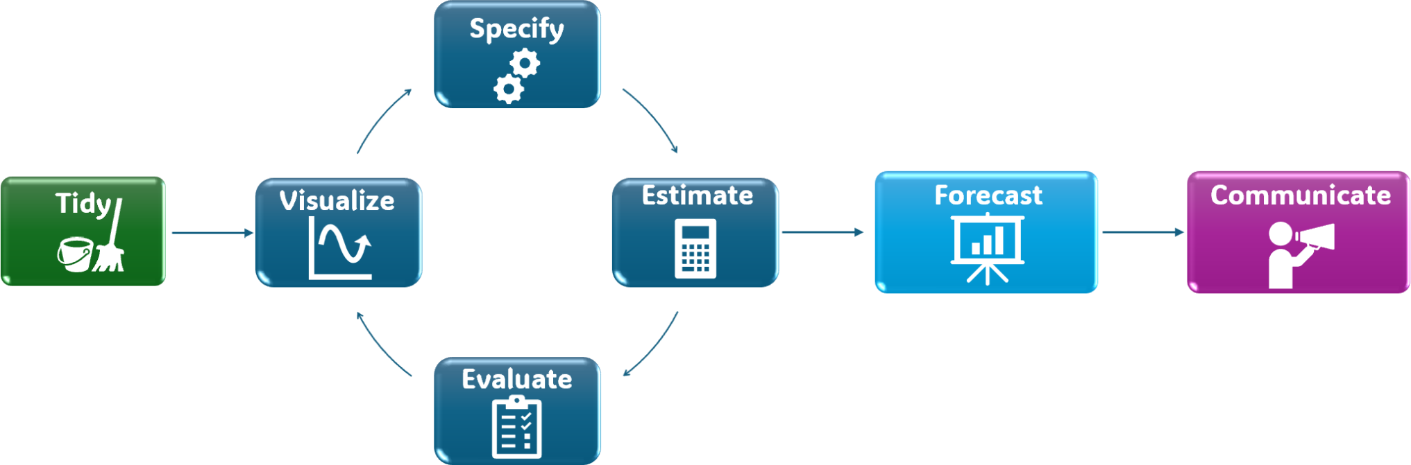
1.0.1 Foundations
Forecasting requires methodological discipline:
- Split the data (train/test)
- Establish benchmark models
- Forecast
- Measure accuracy
- Select a baseline
- Refit and produce the final forecast
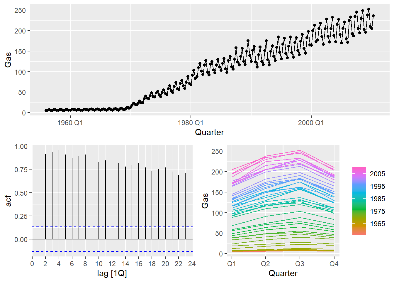
1.0.2 Example dataset
We use a built-in dataset from fpp3: aus_production.
- It is already a
tsibble - It contains multiple economic production series
- We focus on
Gas
1.0.3 Visualize
1.0.4 Train/test split
- Split the series into training and test sets.
- The test set length should match the forecast horizon.
For this example, we use the last 8 quarters as test data.
n_train  n_test
    212       6
NoteSplitting the data
In time series, the training set must contain earlier observations and the test set later observations.
We mimic the real-world scenario: use past data to forecast the future.
1.0.5 Benchmark models
Before fitting complex models, we establish benchmarks.
Common benchmark methods in tidyverts:
- Mean method:
MEAN() - Naïve method:
NAIVE() - Seasonal naïve method:
SNAIVE() - Drift method:
RW(... drift())
Code
bench_fit <- gas_train |>
  model(
    mean   = MEAN(Gas),
    naive  = NAIVE(Gas),
    snaive = SNAIVE(Gas),
    drift  = RW(Gas ~ drift())
  )
1.0.6 Forecast
Generate forecasts with a horizon equal to the test set length.
Code
bench_fcst <- bench_fit |>
  forecast(h = nrow(gas_test))
(Optional) Plot forecasts:
Code
bench_fcst |>
  autoplot(gas_train, level = 95) |>
  autolayer(gas_test, Gas, alpha = 0.7)
1.0.7 Forecast accuracy
We measure forecast accuracy using forecast errors:
e_{T+h} = y_{T+h} - \hat{y}_{T+h|T}
Compute accuracy metrics:
Code
bench_acc <- bench_fcst |>
  accuracy(gas_test) |>
  arrange(MASE)

bench_acc
Selection rule:
- Prefer models that perform well on MASE (scale-independent).
- For seasonal data,
snaiveis often a strong benchmark.
1.0.8 Error metrics
Using forecast errors, we can compute summary metrics:
| Scale | Metric | Description | Formula |
|---|---|---|---|
| Scale-dependent |
|
|
|
| Scale-independent |
|
|
|
1.0.9 Refit and forecast
Once a benchmark is selected based on the test set, refit it using all available data, then forecast the desired future horizon.
Example: refit snaive and forecast the next 8 quarters.
Code
final_fit <- aus_production |>
  model(
    final_model = SNAIVE(Gas)
  )

final_fcst <- final_fit |>
  forecast(h = "8 quarters")
1.0.10 Communicate
Forecasting is not finished when numbers are produced.
Results must be communicated clearly and honestly.
Minimum communication checklist:
- Plot: history + forecast + prediction intervals
- Horizon: what the forecast period represents
- Baseline: state the benchmark model used
- Uncertainty: prediction intervals are essential
- Limitations: structural breaks, short samples, changing conditions