Linear Regression Models for Time Series
The linear model
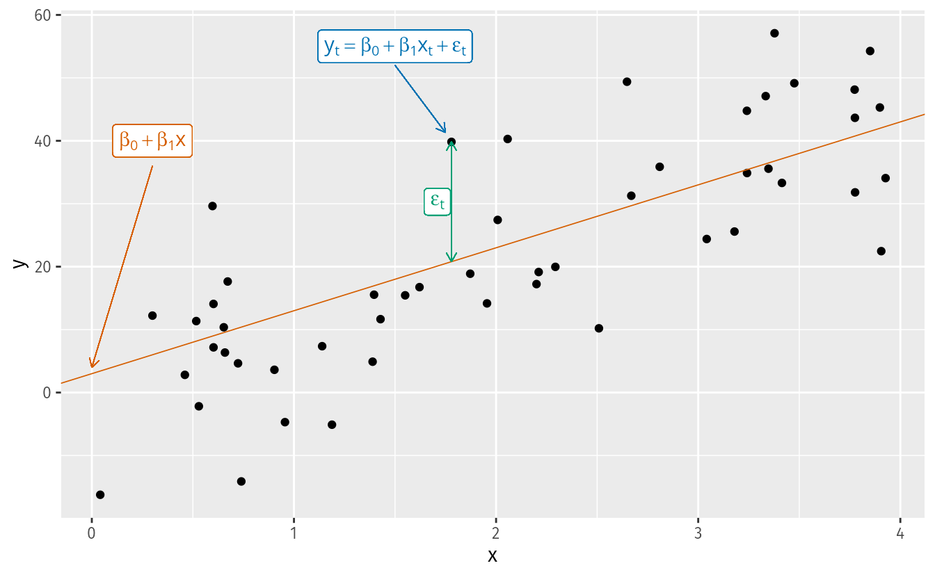
The simplest case is the simple linear regression model:
y_t = \beta_0 + \beta_1 x_t + \varepsilon_t
where:
- \beta_0 is the intercept: the predicted value of y when x = 0.
- \beta_1 is the slope: the average change in y for a one-unit change in x.
- \varepsilon_t is the error term: captures all other influences on y_t not explicitly modeled.
How are the \beta’s estimated? Ordinary Least Squares (OLS)
We cannot observe the \beta’s directly — we estimate them from data. The Ordinary Least Squares (OLS) method chooses the estimates \hat{\beta}_0, \hat{\beta}_1, \ldots, \hat{\beta}_k that minimize the sum of squared residuals:
\min_{\hat{\boldsymbol{\beta}}} \sum_{t=1}^{T} \hat{\varepsilon}_t^2 = \sum_{t=1}^{T} \left(y_t - \hat{\beta}_0 - \hat{\beta}_1 x_{1t} - \cdots - \hat{\beta}_k x_{kt}\right)^2
For the simple case (k = 1), taking partial derivatives and setting them to zero yields closed-form solutions:
\hat{\beta}_1 = \frac{\sum x_t y_t - T\bar{x}\bar{y}}{\sum x_t^2 - T\bar{x}^2}, \qquad \hat{\beta}_0 = \bar{y} - \hat{\beta}_1 \bar{x}
For the general case with k predictors, the solution extends naturally to matrix form:
\hat{\boldsymbol{\beta}} = (\mathbf{X}^\top \mathbf{X})^{-1} \mathbf{X}^\top \mathbf{y}
where \mathbf{X} is the design matrix — a column of ones (for the intercept) plus one column per predictor — and \mathbf{y} is the vector of observed responses.
In practice, R handles all of this internally. But knowing the objective function matters: OLS penalizes large residuals more than small ones (because of the square), and under the classical assumptions the Gauss-Markov theorem guarantees the estimates are BLUE (Best Linear Unbiased Estimators) — regardless of whether we have one predictor or twenty.
Real examples
- Ice cream sales (y) and daily temperature (x).
- Nike revenue (y) and marketing spend (x).
- US consumption growth (y) and income growth (x).
- Mexico retail trade (y) and consumer confidence index (x).
Terminology: many names for y and x
The same concept appears under different names depending on the discipline:
| y (forecast variable) | x (predictor variables) |
|---|---|
| Dependent | Independent |
| Explained | Explanatory |
| Regressand | Regressor |
| Response | Stimulus / Covariate |
| Endogenous | Exogenous |
In time series forecasting, FPP3 uses forecast variable and predictor variables.
The origin of “regression” — Galton, 1886
The term was coined by Francis Galton while studying the relationship between parents’ height and their children’s height.
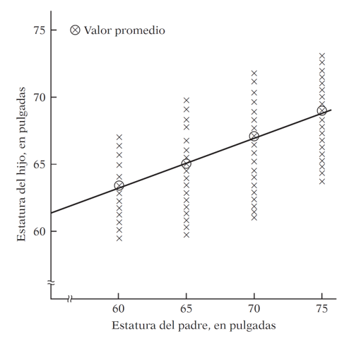
His finding: tall parents tend to have tall children, but on average their children are not as tall as them. Short parents tend to have children taller than themselves. There is a tendency to regress toward the mean.
Without this regression to the mean, the distribution of heights across generations would diverge — we would eventually have people of Hobbit stature and people of giant stature, with nothing in between.
Modern regression analysis generalizes this idea: studying the dependence of one variable on one or more others to predict its average value.
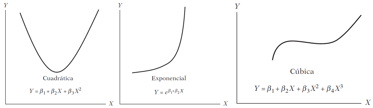
Are these models linear?
Exploratory analysis
Before fitting any model, we look at the data.
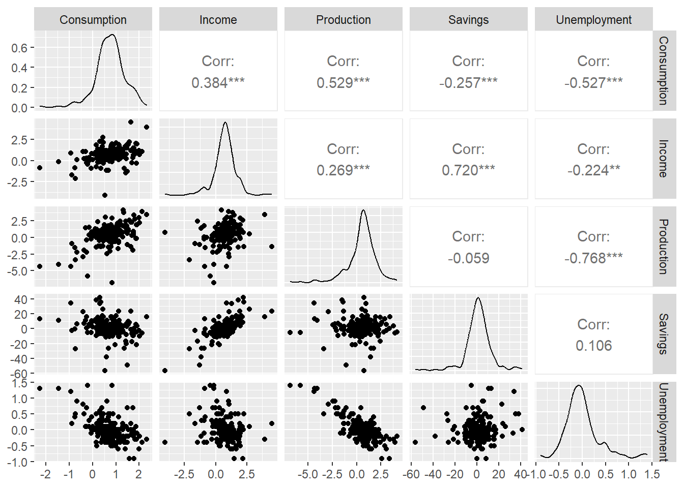
The scatter matrix shows correlations between all pairs of variables. Notice that some predictors are correlated with each other — we will return to this when we discuss multicollinearity.
Residual Diagnostics
Gauss-Markov assumptions and why they matter in time series
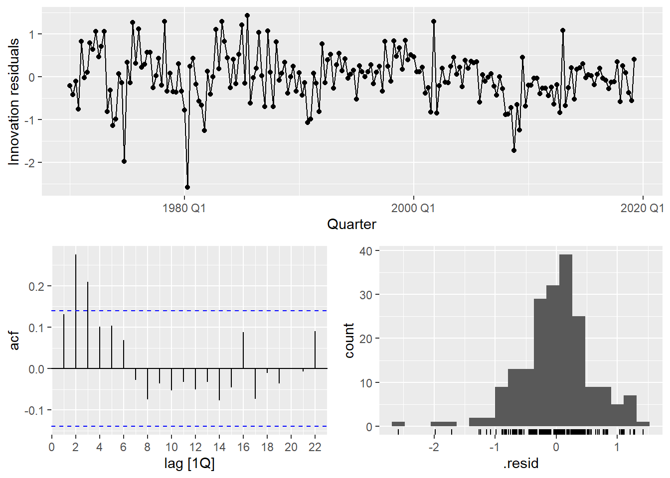
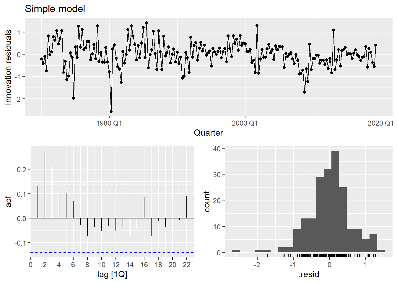
OLS produces BLUE estimators only if the classical assumptions hold. The one most frequently violated in time series is no autocorrelation in the errors:
\text{cov}(\varepsilon_t, \varepsilon_s) = 0 \quad \forall \; t \neq s
If residuals are autocorrelated, OLS estimates are still unbiased but no longer efficient — standard errors are wrong, p-values are wrong, and forecast intervals are wrong. This is why we always check the residuals.
- 1
- Extract the number of estimated parameters to use as degrees of freedom correction.
- 2
- A significant p-value indicates autocorrelated residuals — a sign the model is missing structure.
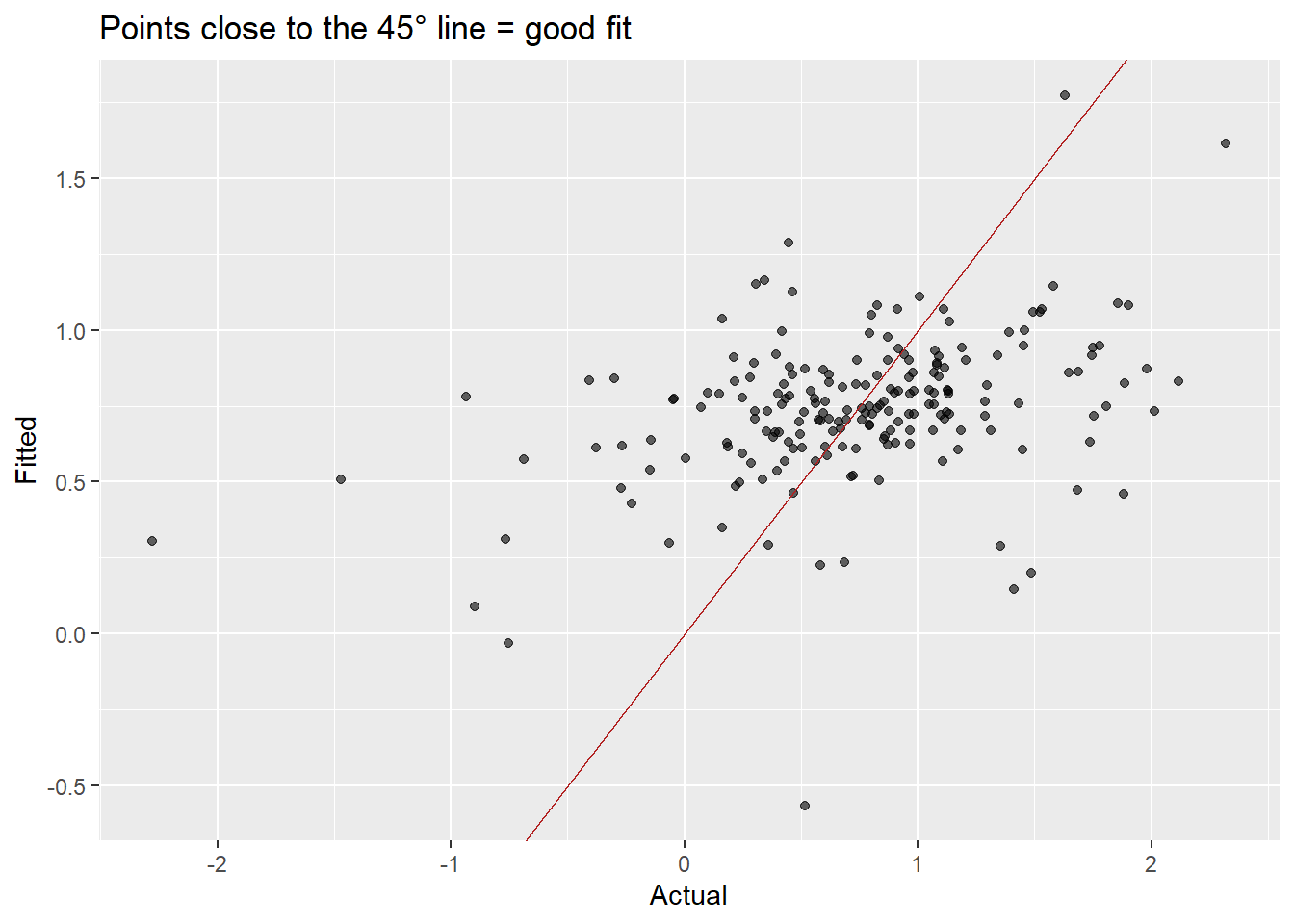
The residuals show clear autocorrelation. The simple model is not capturing all the dynamics of consumption. Let’s improve it.
Comparing simple vs. multiple
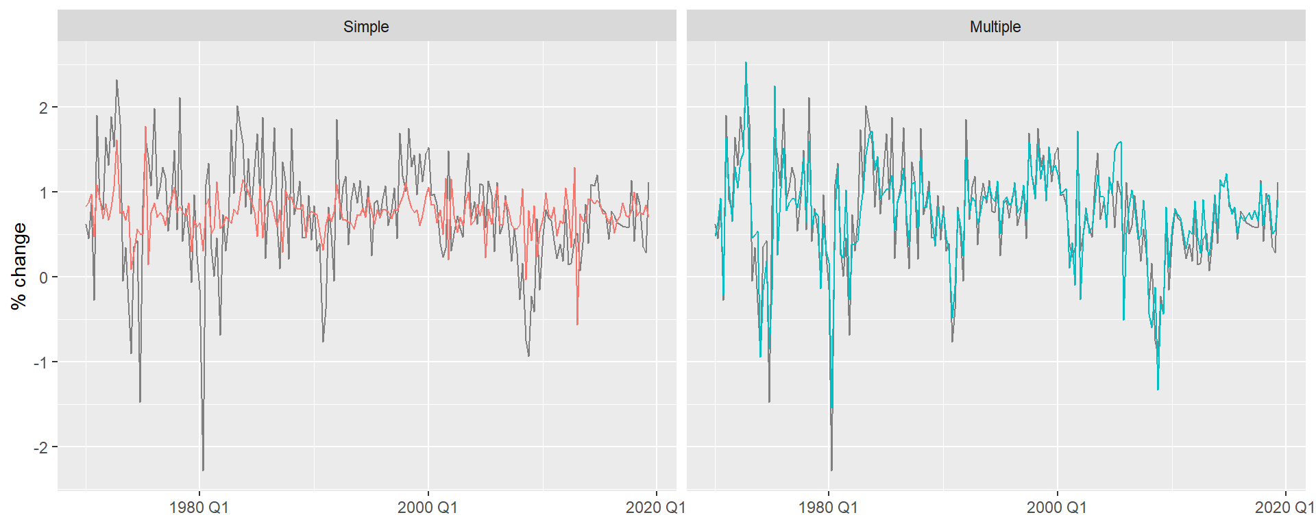

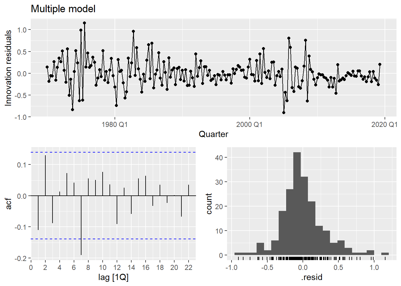
The multiple model substantially improves fit (\bar{R}^2 goes from ~0.15 to ~0.75) and the residuals look much closer to white noise.
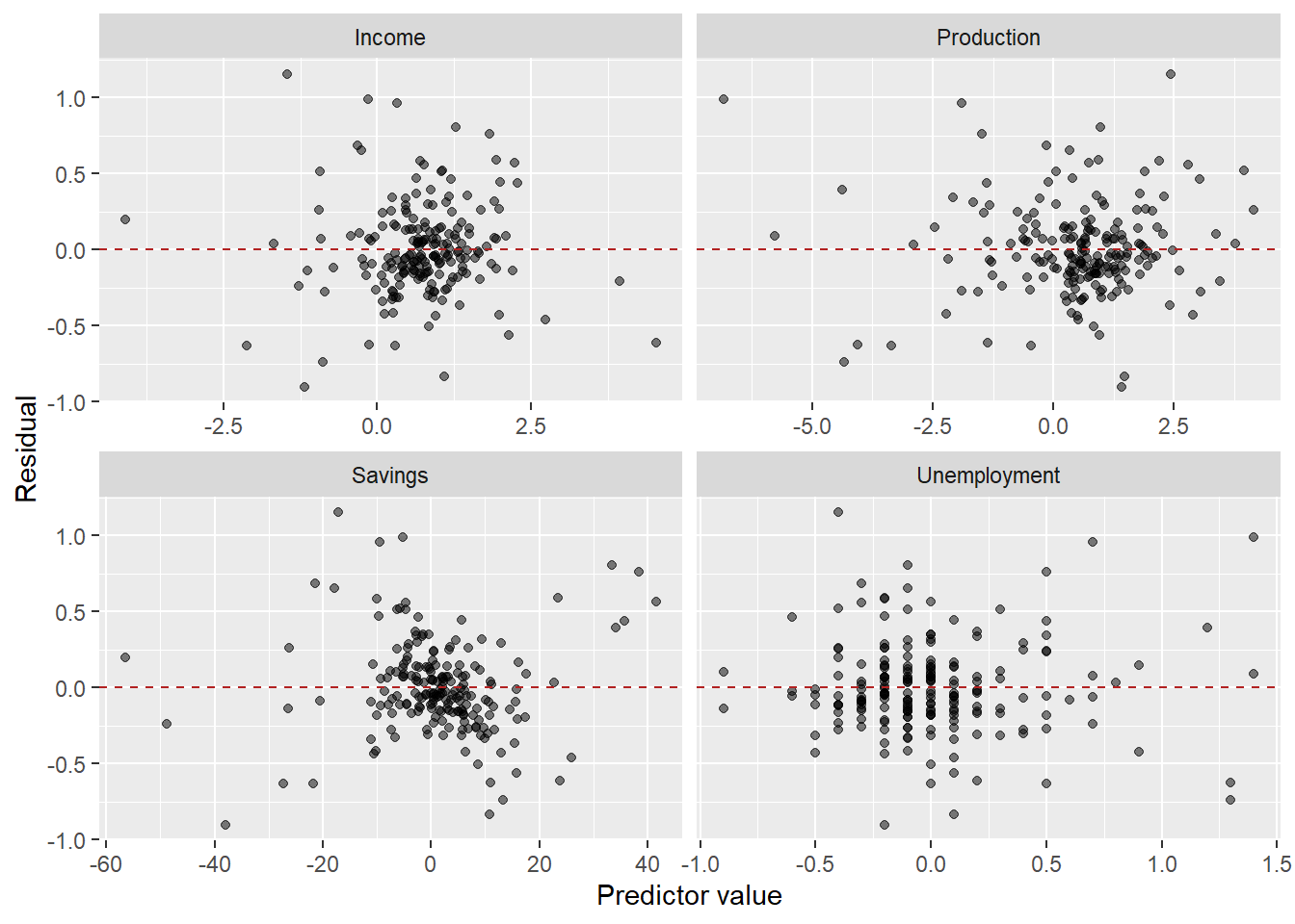
The residuals vs. predictors plot is a useful diagnostic specific to multiple regression. If any panel shows a systematic pattern (curve, fan shape), it suggests a missing nonlinear term or interaction involving that predictor.
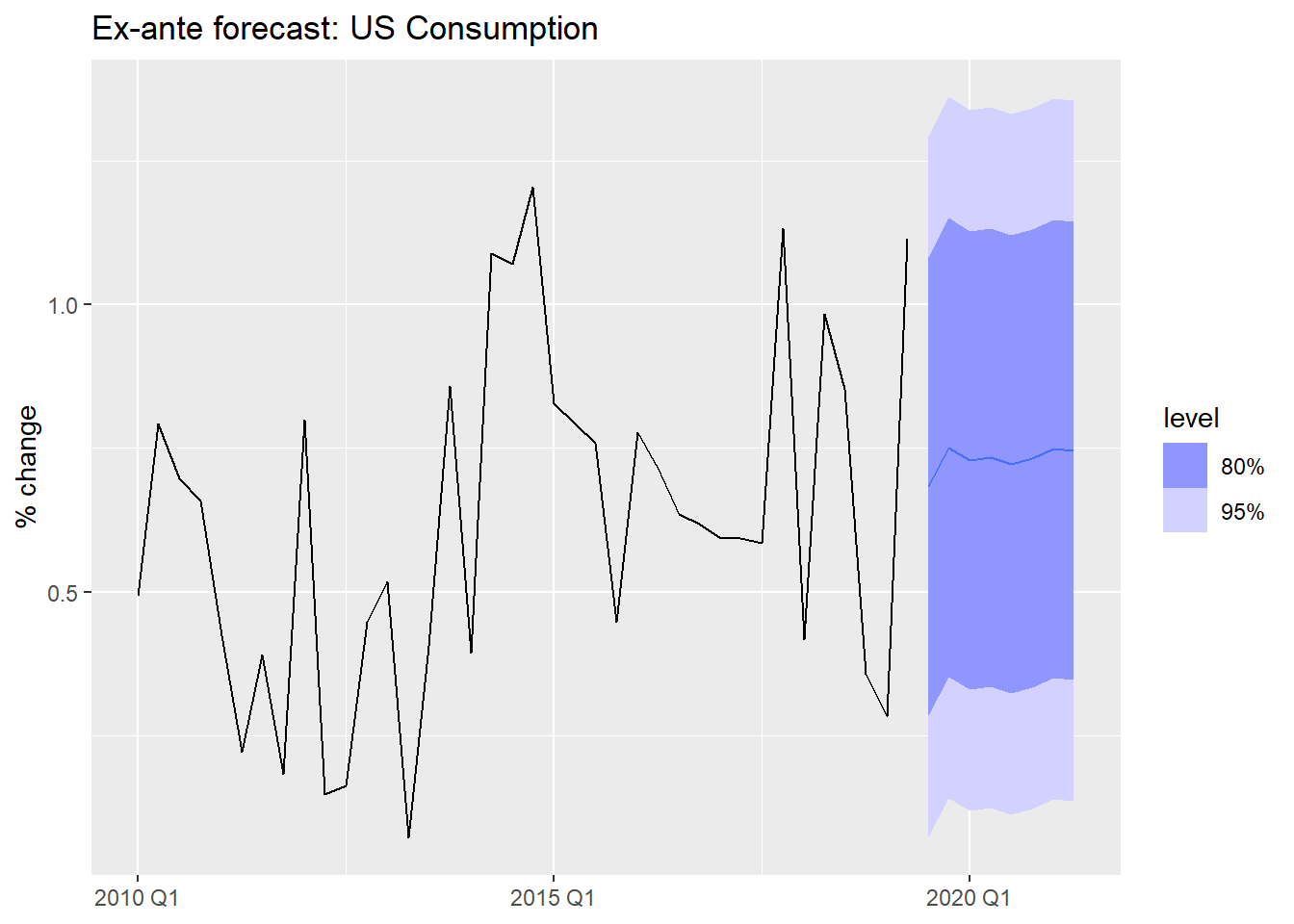
Three types of forecasts
Ex-ante forecasts use only information available at the time the forecast is made. The predictors must themselves be forecasted.
This is the “true” forecast — it is what you would actually produce in a real deployment.
us_change_future <- us_change |>
pivot_longer(-c(Quarter, Consumption), names_to = "variable") |>
model(arima = ARIMA(value)) |>
forecast(h = 8) |>
as_tsibble() |>
select(-c(.model, value)) |>
pivot_wider(names_from = variable, values_from = .mean)
us_change_fit_mult |>
forecast(new_data = us_change_future) |>
autoplot(us_change |> filter_index("2010 Q1" ~ .)) +
labs(title = "Ex-ante forecast: US Consumption",
y = "% change", x = NULL)- 1
-
Pivot to long format — each predictor becomes a separate series keyed by
variable. - 2
-
A single
model()call fits an ARIMA to each predictor automatically. - 3
-
A single
forecast()produces 8-step-ahead forecasts for all predictors simultaneously. - 4
-
Convert back to tsibble — required by
forecast()when passed asnew_data. - 5
- Pivot back to wide so each predictor has its own column, matching the structure expected by the regression model.
Ex-post forecasts use actual realized values of the predictors. The forecast variable y_t is still unknown, but we feed in the true future x_t values.
These are not “real” forecasts — they are used to evaluate the regression model in isolation, removing predictor forecast error from the evaluation.
# Use filter_index to create a train/test split
us_change_train <- us_change |>
  filter_index(. ~ "2017 Q4")

us_change_test <- us_change |>
  filter_index("2018 Q1" ~ .)

us_change_fit_expost <- us_change_train |>
  model(
    multiple = TSLM(Consumption ~ Income + Production + Savings + Unemployment)
  )

# Ex-post: we supply actual future predictor values
us_change_fit_expost |>
  forecast(new_data = us_change_test) |>
  autoplot(us_change |> filter_index("2014 Q1" ~ .)) +
  labs(title = "Ex-post forecast: actual predictor values used",
       y = "% change", x = NULL)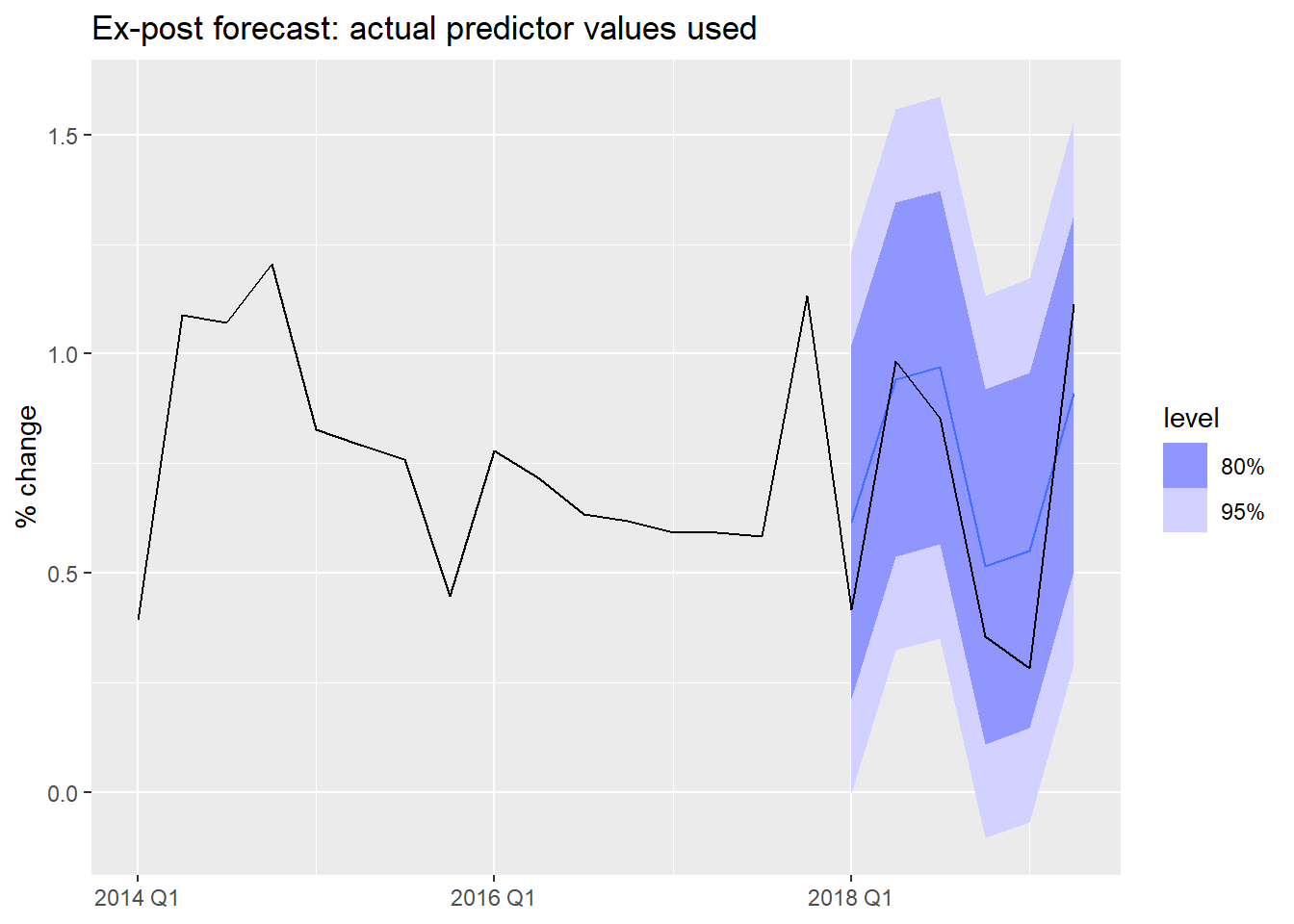
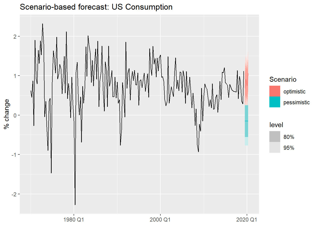
Scenario-based forecasts construct hypothetical future values for the predictors and ask: what would consumption look like under each scenario?
These are especially useful for stress-testing and strategic planning.
us_change_fit_scen <- us_change |>
model(TSLM(Consumption ~ Income + Savings + Unemployment))
us_change_scenarios <- scenarios(
optimistic = new_data(us_change, 4) |>
mutate(Income = c(0.5, 0.8, 0.6, 1.0),
Savings = c(0.1, -0.2, 0.1, -0.1),
Unemployment = -0.1),
pessimistic = new_data(us_change, 4) |>
mutate(Income = -0.5,
Savings = -0.4,
Unemployment = 0.2),
names_to = "Scenario"
)
us_change |>
autoplot(Consumption) +
autolayer(forecast(us_change_fit_scen, new_data = us_change_scenarios)) +
labs(title = "Scenario-based forecast: US Consumption",
y = "% change", x = NULL)- 1
- We fit a simpler model using only the three predictors with clearest economic interpretation.
- 2
- Optimistic scenario: income grows steadily, savings fluctuate mildly, unemployment falls slightly.
- 3
- Pessimistic scenario: income contracts, savings decline, unemployment rises.
- 4
-
names_tolabels each scenario in the output, making it easy to distinguish them in the plot. - 5
-
autolayer()overlays the scenario forecasts on the historical series without requiring matching key structures.
Can regression handle trend and seasonality?
We have seen regression with exogenous variables. But can TSLM() also handle the patterns we identified in Module 1 — trend and seasonality?
Yes — through specially constructed predictors built directly into the formula.
We will illustrate with quarterly beer production in Australia.
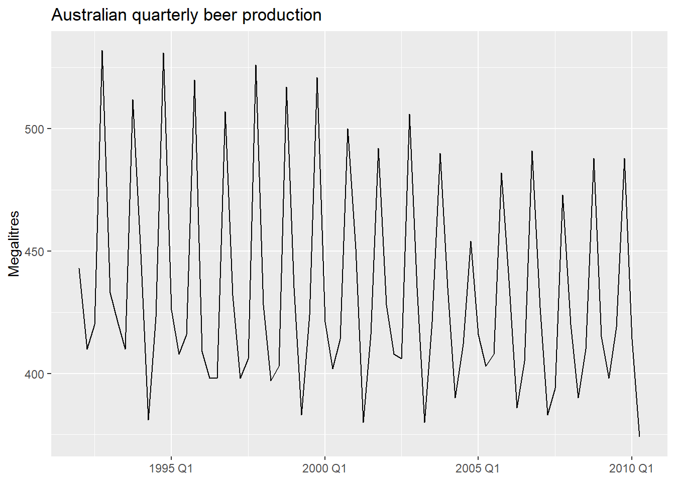
Trend and seasonal dummies in R
TSLM() provides two built-in terms:
trend()— a deterministic linear trend: \beta_1 t where t = 1, 2, \ldots, T.season()— m - 1 seasonal dummy variables, with the first season as baseline.
- 1
-
trend()adds a linear time index;season()adds quarterly dummies automatically.
Series: Beer
Model: TSLM

Residuals:
     Min       1Q   Median       3Q      Max
-42.9029  -7.5995  -0.4594   7.9908  21.7895

Coefficients:
               Estimate Std. Error t value Pr(>|t|)
(Intercept)   441.80044    3.73353 118.333  < 2e-16 ***
trend()        -0.34027    0.06657  -5.111 2.73e-06 ***
season()year2 -34.65973    3.96832  -8.734 9.10e-13 ***
season()year3 -17.82164    4.02249  -4.430 3.45e-05 ***
season()year4  72.79641    4.02305  18.095  < 2e-16 ***
---
Signif. codes:  0 '***' 0.001 '**' 0.01 '*' 0.05 '.' 0.1 ' ' 1

Residual standard error: 12.23 on 69 degrees of freedom
Multiple R-squared: 0.9243, Adjusted R-squared: 0.9199
F-statistic: 210.7 on 4 and 69 DF, p-value: < 2.22e-16
What about more complex seasonality? Fourier terms
For series with multiple seasonal periods or very long seasons (daily, hourly data), season() becomes impractical — the number of dummies grows too large. An alternative is Fourier terms: pairs of sine and cosine waves that approximate the seasonal pattern with far fewer parameters.
TSLM() supports this via fourier(K), where K controls how many Fourier pairs are included. We will cover this properly in Module 4 when we deal with complex seasonality.
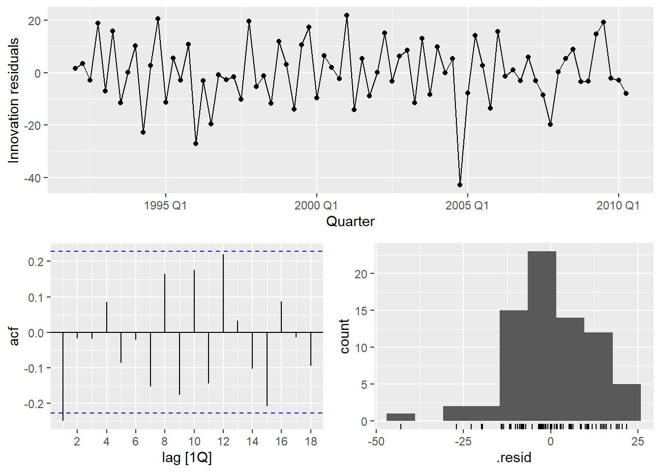
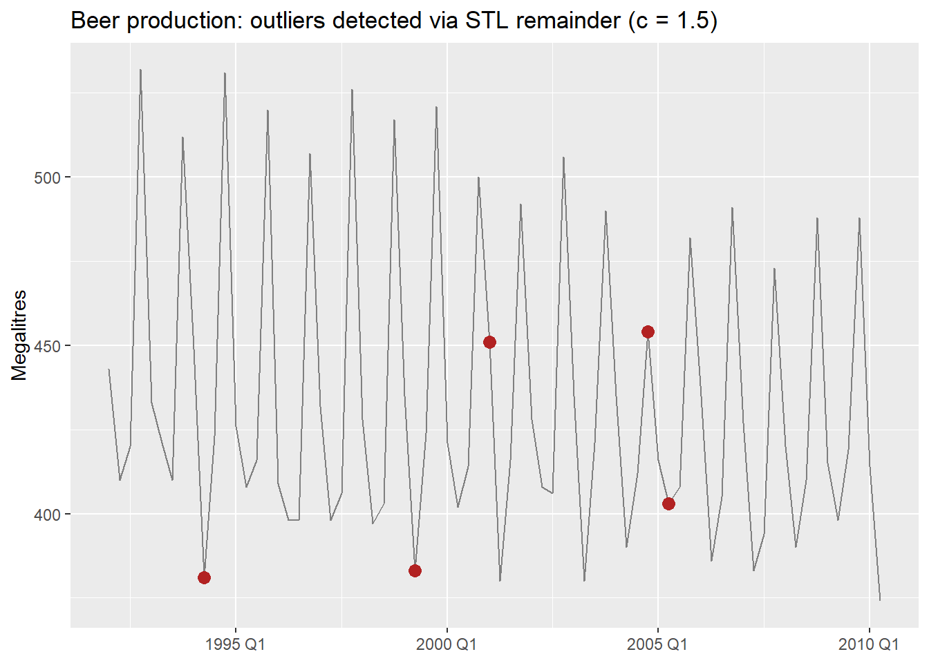
There is a notable outlier in Q2 1994. We can detect it formally and then handle it with an intervention variable.
Intervention Variables and Outliers
Formal outlier detection
Rather than eyeballing the residual plot, we can detect outliers formally — the same way we did in the practical issues document. The key idea is that applying the IQR rule directly to the raw series does not work in time series: a series with trend has naturally increasing values, so later observations always look “large” even when they are perfectly normal.
The fix: decompose first, then apply IQR to the remainder. For beer, which has strong known seasonality, we use a full STL decomposition — including the seasonal component — so only genuine anomalies end up in the remainder1.
beer_dcmp <- beer |>
model(
stl = STL(Beer ~ trend() + season(), robust = TRUE)
) |>
components()
beer_outliers <- beer_dcmp |>
select(Quarter, remainder) |>
mutate(
Q1 = quantile(remainder, 0.25),
Q3 = quantile(remainder, 0.75),
IQR = Q3 - Q1,
lower_15 = Q1 - 1.5 * IQR,
upper_15 = Q3 + 1.5 * IQR,
lower_3 = Q1 - 3 * IQR,
upper_3 = Q3 + 3 * IQR,
outlier_15 = remainder < lower_15 | remainder > upper_15,
outlier_3 = remainder < lower_3 | remainder > upper_3
)
beer_outliers |>
filter(outlier_15) |>
select(Quarter, remainder, outlier_15, outlier_3)- 1
-
Full STL with both trend and season — for a strongly seasonal series like
beer, this prevents normal seasonal variation from being flagged as anomalies. - 2
- Standard threshold (c = 1.5): flags moderate outliers.
- 3
- Stricter threshold (c = 3): flags only extreme observations. Use this when you want to be conservative.
Types of intervention variables
In regression, rather than removing the outlier and imputing, we model it explicitly with a dummy variable. This keeps all observations and lets the model account for the anomaly without distorting the other coefficients.
- Spike variable: 1 for a single anomalous period, 0 everywhere else. Captures a one-off shock.
- Level shift variable: 0 before an event, 1 from the event onward. Captures a permanent change in level.
- Ramp variable: 0 before an event, then increasing linearly. Captures a gradual structural shift.
- 1
- Spike: 1 only in 1994 Q2, captures the single anomalous quarter.
- 2
- Level shift: 1 from year 2000 onward, allows a different intercept from that point.
Series: Beer
Model: TSLM

Residuals:
     Min       1Q   Median       3Q      Max
-42.7196  -6.9594  -0.7748   8.0050  21.5292

Coefficients:
              Estimate Std. Error t value Pr(>|t|)
(Intercept)   442.6530     3.8050 116.336  < 2e-16 ***
trend()        -0.3730     0.1285  -2.902  0.00501 **
season()year2 -33.3328     3.9745  -8.387 4.84e-12 ***
season()year3 -17.8072     3.9716  -4.484 2.95e-05 ***
season()year4  72.8436     3.9773  18.315  < 2e-16 ***
spike_Q2_1994 -24.5904    12.5547  -1.959  0.05432 .
level_2000      0.6182     5.5264   0.112  0.91127
---
Signif. codes:  0 '***' 0.001 '**' 0.01 '*' 0.05 '.' 0.1 ' ' 1

Residual standard error: 12.07 on 67 degrees of freedom
Multiple R-squared: 0.9284, Adjusted R-squared: 0.922
F-statistic: 144.9 on 6 and 67 DF, p-value: < 2.22e-16
We will revisit outlier handling in Module 4, where we cover robust methods and automatic outlier detection. Intervention variables are the regression-world equivalent of those techniques — explicit rather than automatic.
Piecewise Linear Trends
When the trend changes slope at one or more points in time, a piecewise linear model fits separate linear segments joined at knots.
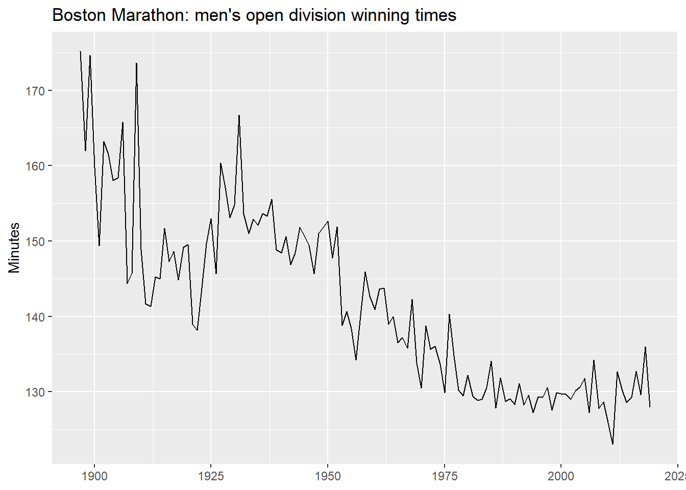
We use the Boston Marathon winning times — a series with clear structural breaks.
A linear trend first
What does a single linear trend produce on this data?
boston_fit_linear <- boston_men |>
  model(linear = TSLM(Minutes ~ trend()))

boston_men |>
  autoplot(Minutes, color = "grey60") +
  geom_line(
    data = fitted(boston_fit_linear),
    aes(y = .fitted), color = "#0072B2"
  ) +
  autolayer(forecast(boston_fit_linear, h = 10),
            alpha = 0.5, level = 95) +
  labs(title = "Boston Marathon: linear trend",
       y = "Minutes", x = NULL)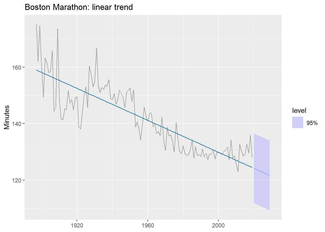
The forecast predicts times will keep falling indefinitely — eventually reaching zero. A single linear trend is the wrong functional form here.
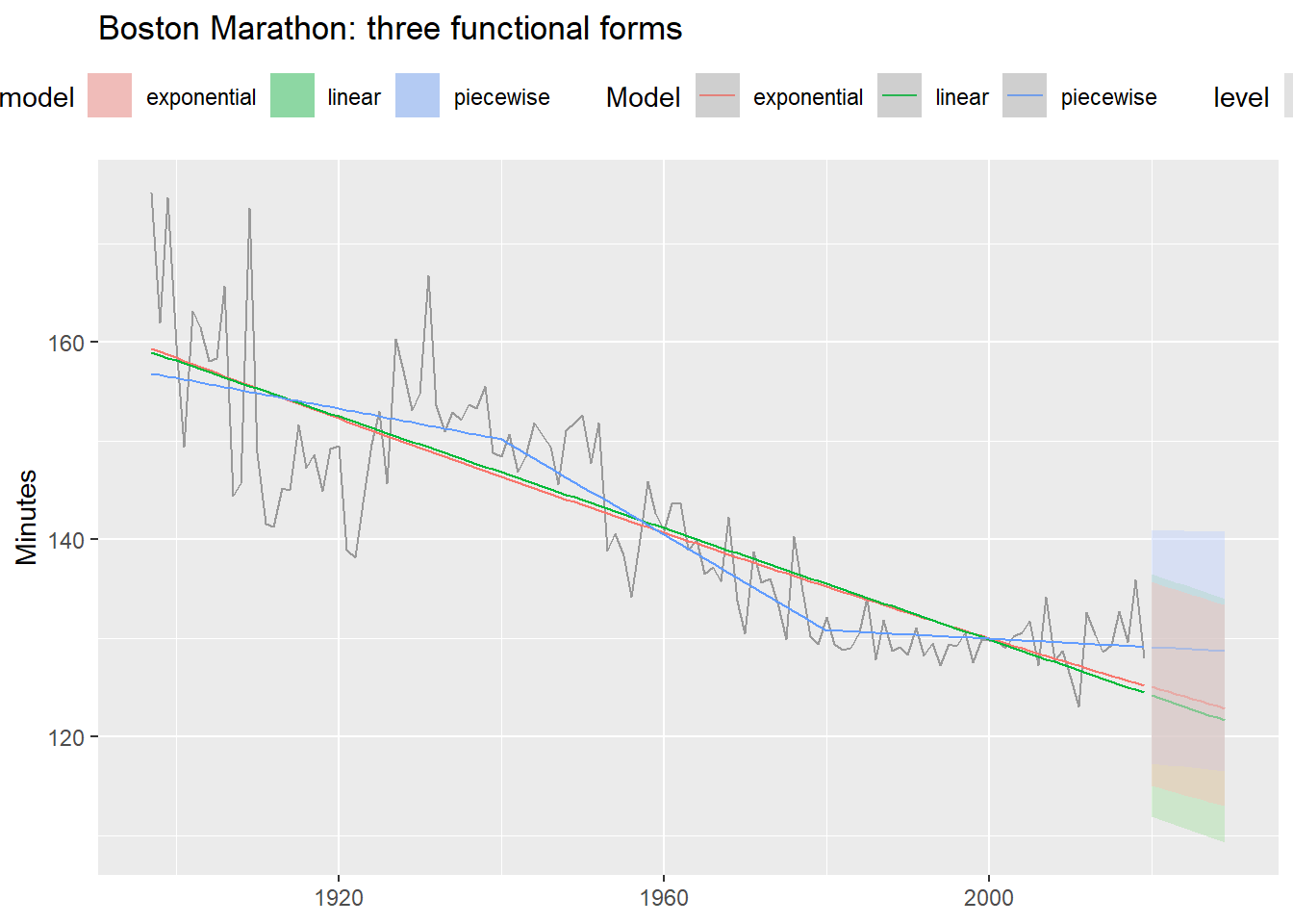
Three functional forms
boston_fit <- boston_men |>
model(
linear = TSLM(Minutes ~ trend()),
exponential = TSLM(log(Minutes) ~ trend()),
piecewise = TSLM(Minutes ~ trend(knots = c(1940, 1980)))
)
boston_men |>
autoplot(Minutes, color = "grey60") +
geom_line(
data = fitted(boston_fit),
aes(y = .fitted, color = .model)
) +
autolayer(forecast(boston_fit, h = 10),
alpha = 0.4, level = 95) +
labs(title = "Boston Marathon: three functional forms",
y = "Minutes", x = NULL, color = "Model") +
theme(legend.position = "top")- 1
- Log-transformed response: assumes times decrease at a declining rate.
- 2
-
knotsspecify the years where the slope is allowed to change.
The knot selection problem
A key limitation of piecewise regression: we must choose the knots ourselves. Different choices can produce very different forecasts, even when in-sample fit looks similar.
boston_fit_knots <- boston_men |>
  model(
    k1 = TSLM(Minutes ~ trend(knots = c(1940, 1980))),
    k2 = TSLM(Minutes ~ trend(knots = c(1915, 1950))),
    k3 = TSLM(Minutes ~ trend(knots = c(1950, 1970, 1990)))
  )

boston_men |>
  autoplot(Minutes, color = "grey60") +
  geom_line(
    data = fitted(boston_fit_knots),
    aes(y = .fitted, color = .model)
  ) +
  autolayer(forecast(boston_fit_knots, h = 10),
            alpha = 0.4, level = 95) +
  labs(title = "Different knots → very different forecasts",
       y = "Minutes", x = NULL, color = "Model") +
  theme(legend.position = "top")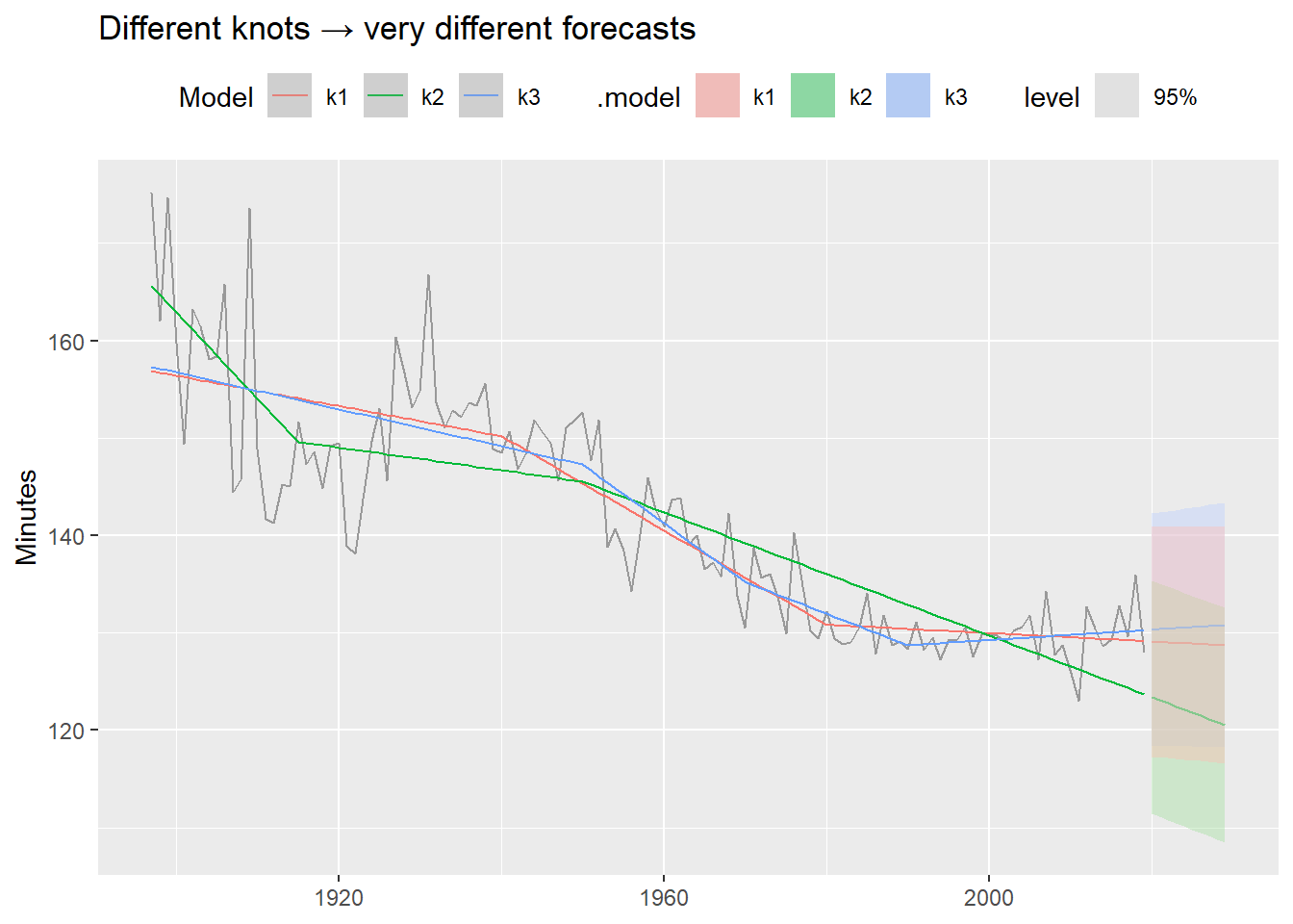
These models fit the historical data similarly well — but their forecasts diverge dramatically. Always inspect the forecast, not just the in-sample fit. This is one motivation for Prophet (Module 4), which detects changepoints automatically from the data rather than requiring manual specification.
Footnotes
When seasonality is weak or absent,
season(period = 1)can be used to extract only the trend. See Practical Forecasting Issues for the full workflow including NA imputation.