- 1
-
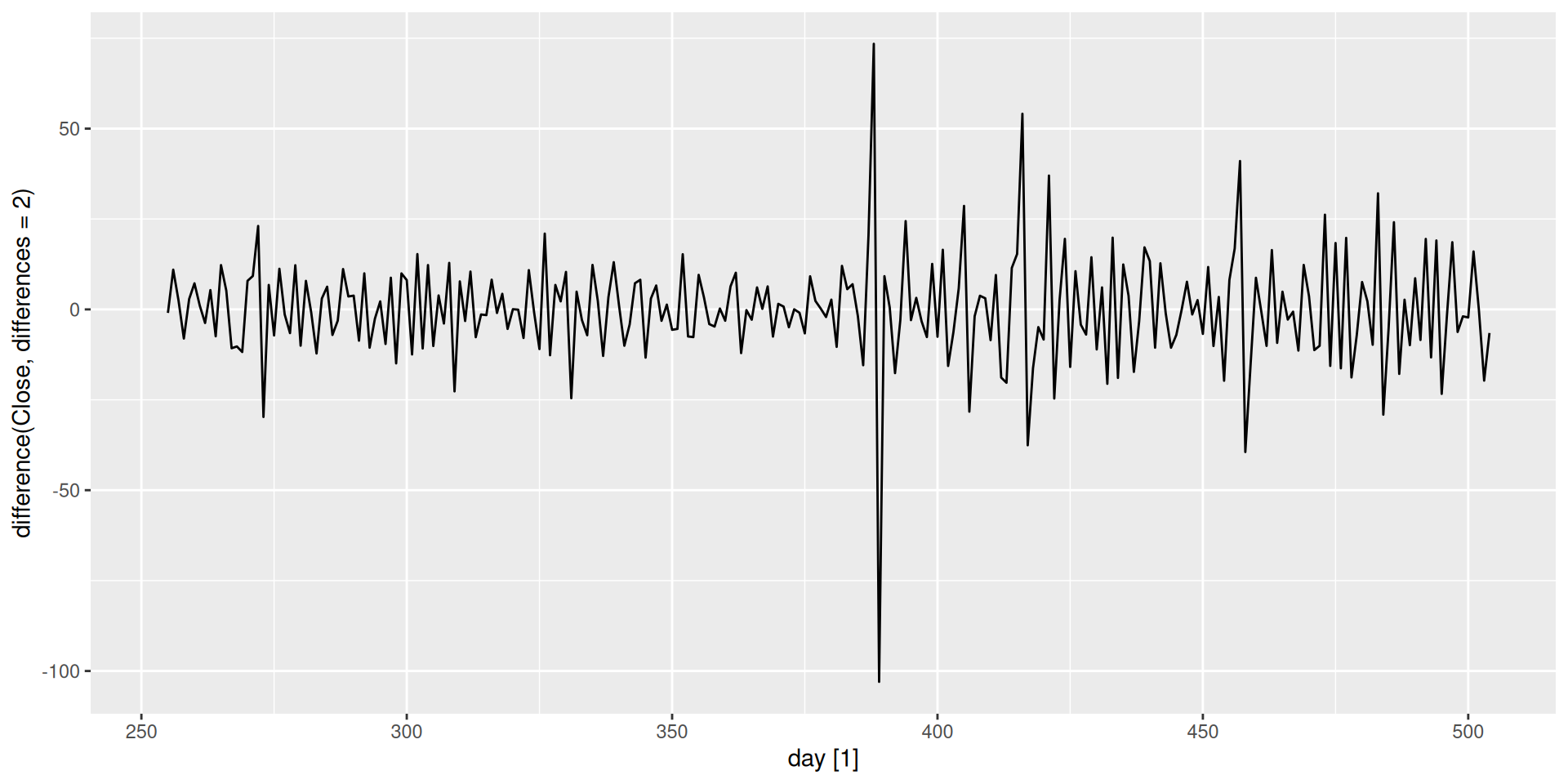
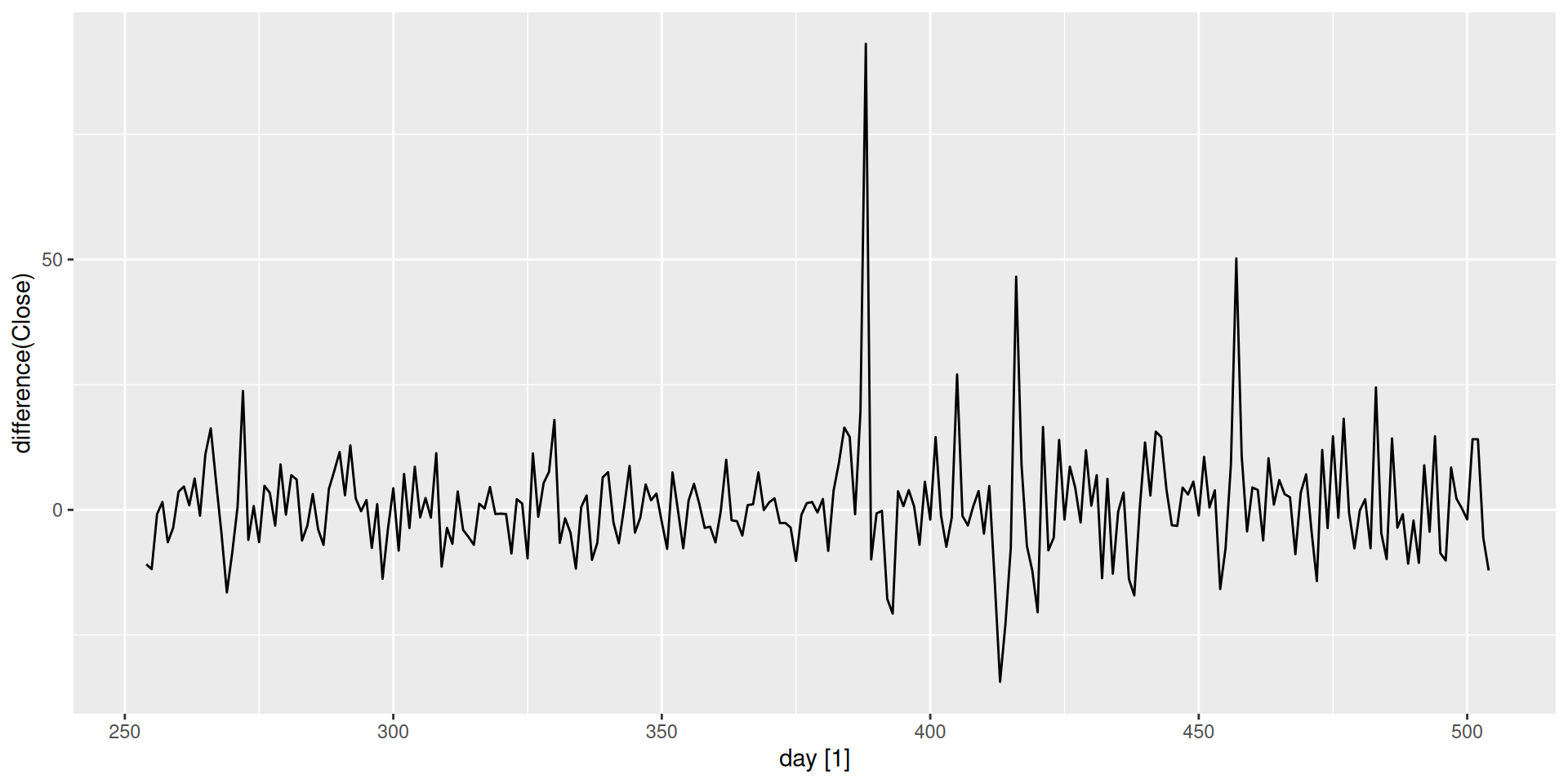
difference(Close)computes the first difference of theClosevariable.
Have you ever heard the word “stationary” before?

Think about it
If a time series is “not moving”, what statistical properties would you expect it to have?
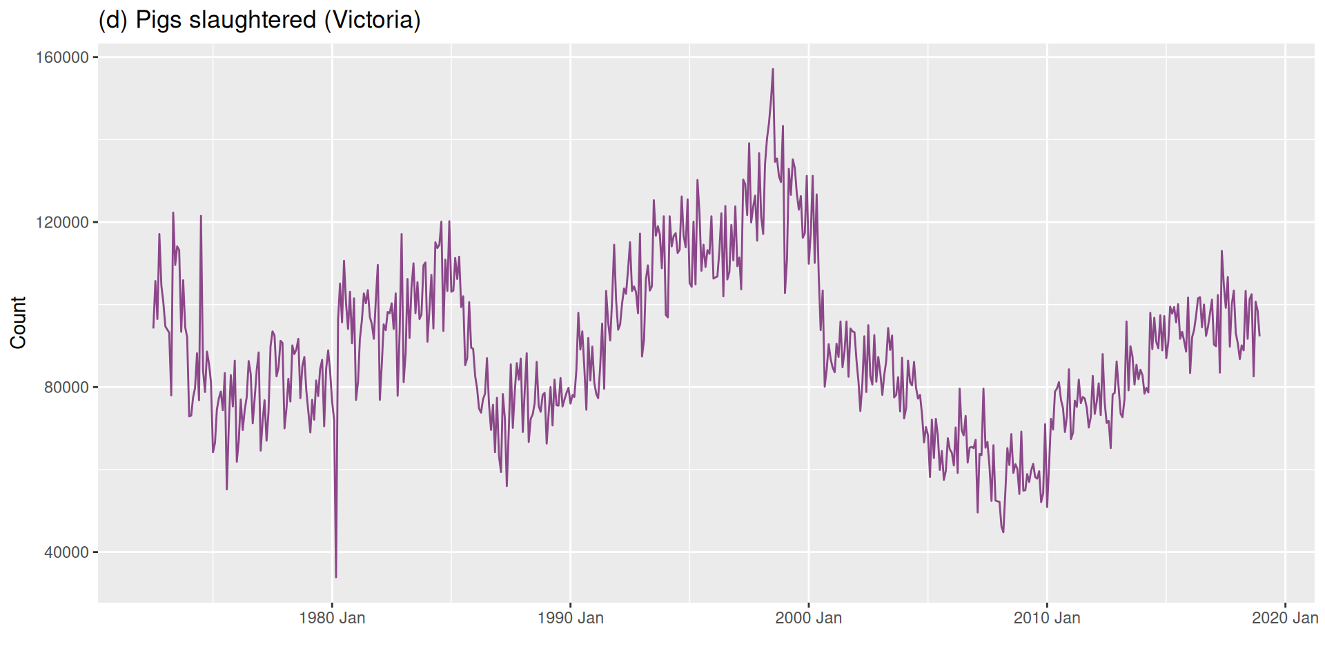
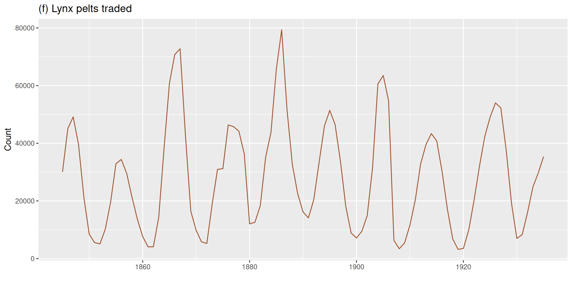
Which of the following six series are stationary (i.e., which look more stable)?

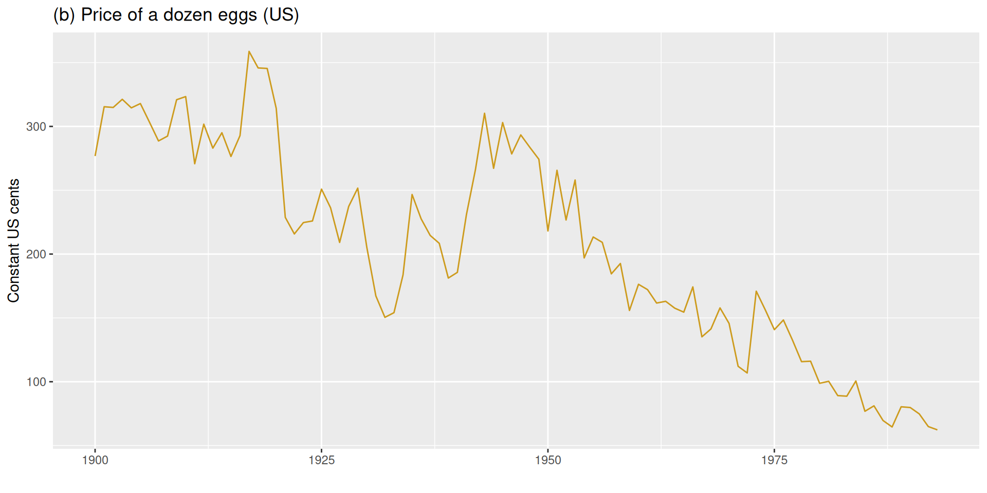
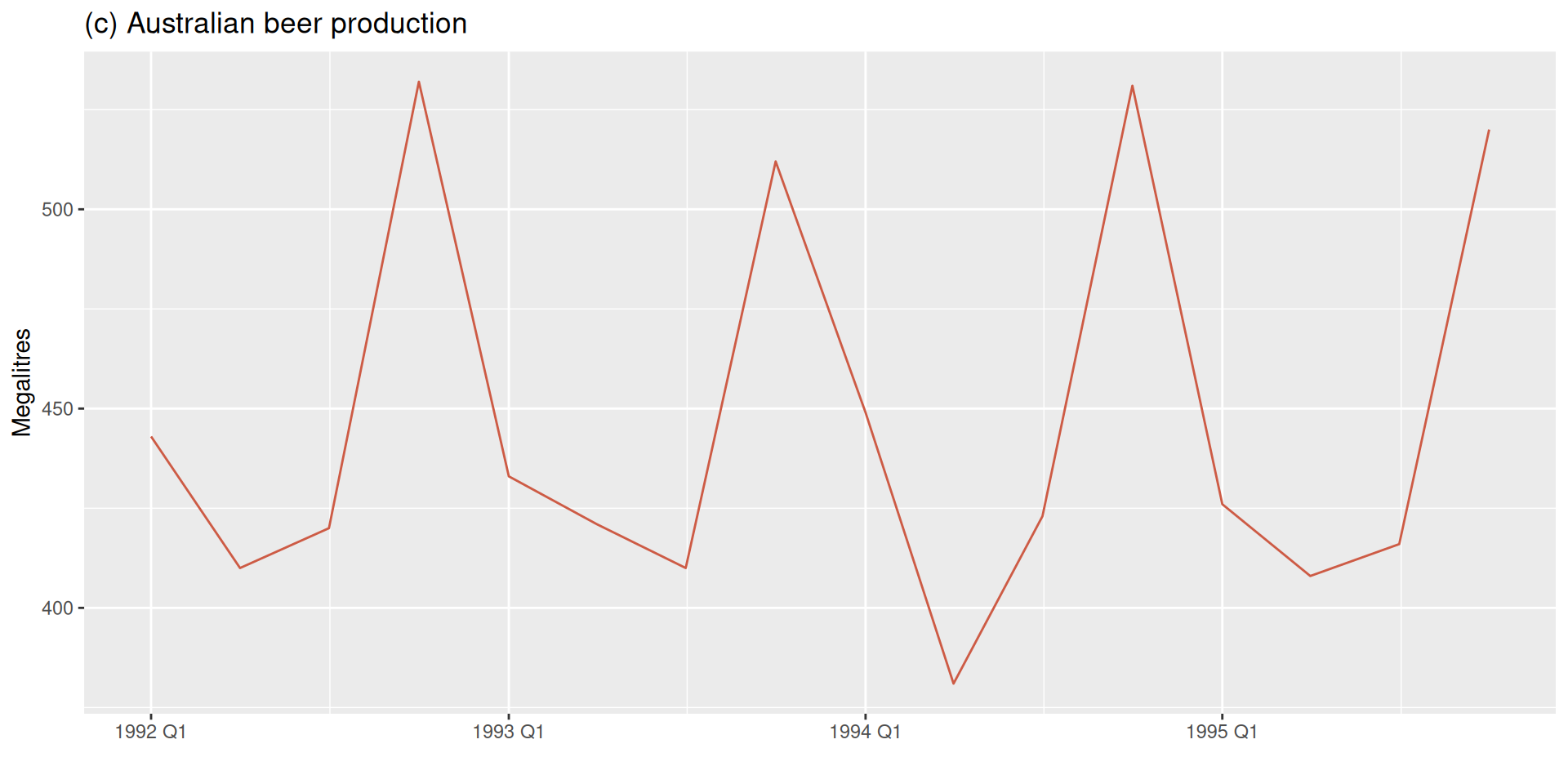

Look at these two series:
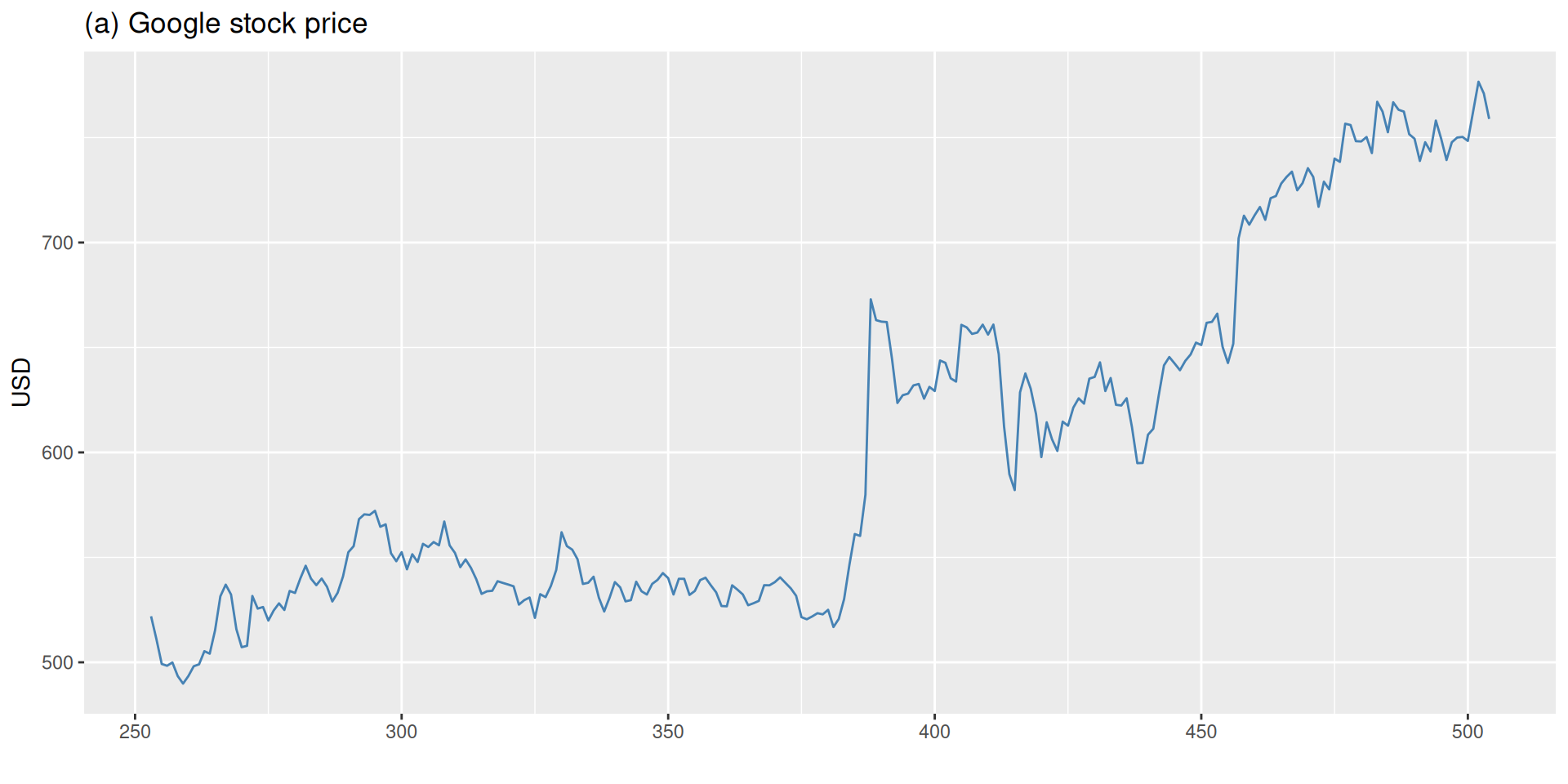
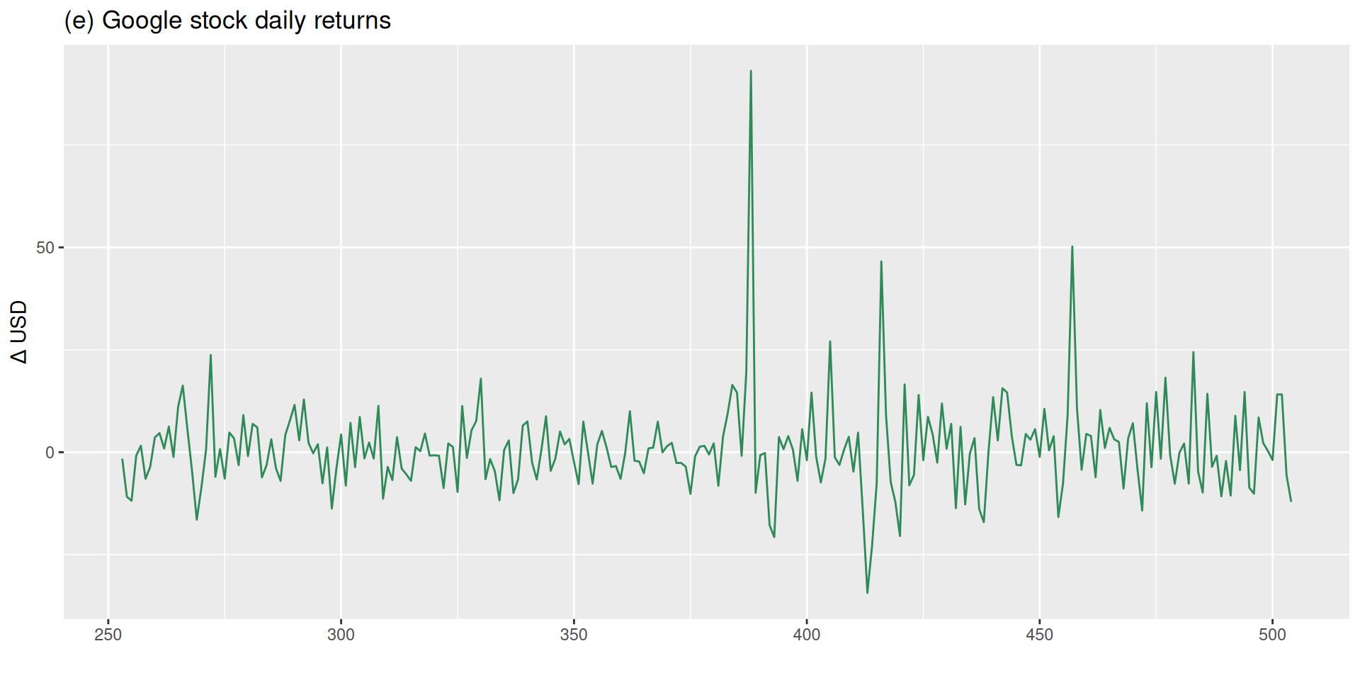
The second series was produced directly from the first. Can you figure out how?
Differencing
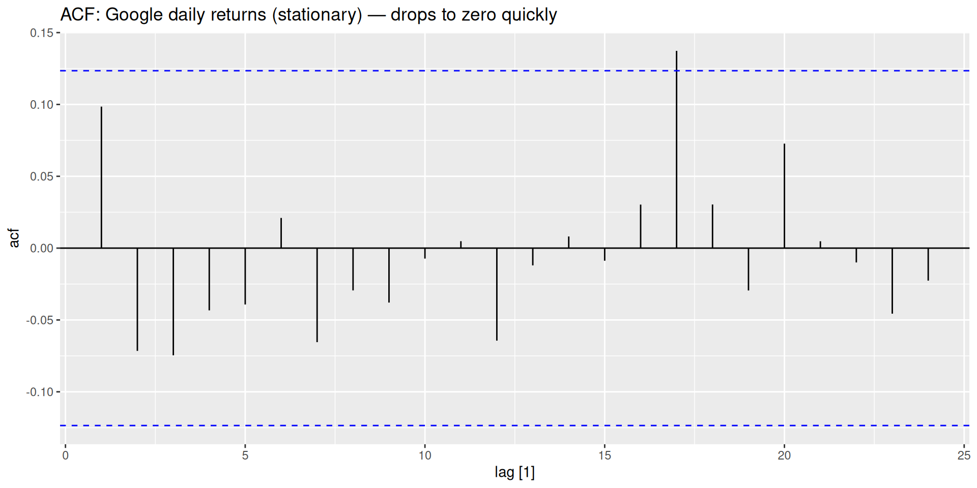
The daily return is simply today’s price minus yesterday’s price — the change between consecutive observations. This operation is called differencing, and it is how we stabilize the mean of a non-stationary series.
Random walks & stationarity
The first difference of a series y_t is:
y'_t = y_t - y_{t-1}
Sometimes the first-differenced series is still non-stationary. We can difference again:
\begin{align*} y''_t &= y'_t - y'_{t-1} \\ &= (y_t-y_{t-1}) - (y_{t-1} - y_{t-2}) \\ &= y_t - 2y_{t-1} + y_{t-2} \end{align*}
Needing three or more differences usually signals something else is wrong — an outlier, a structural break, or a transformation that should have been applied first.
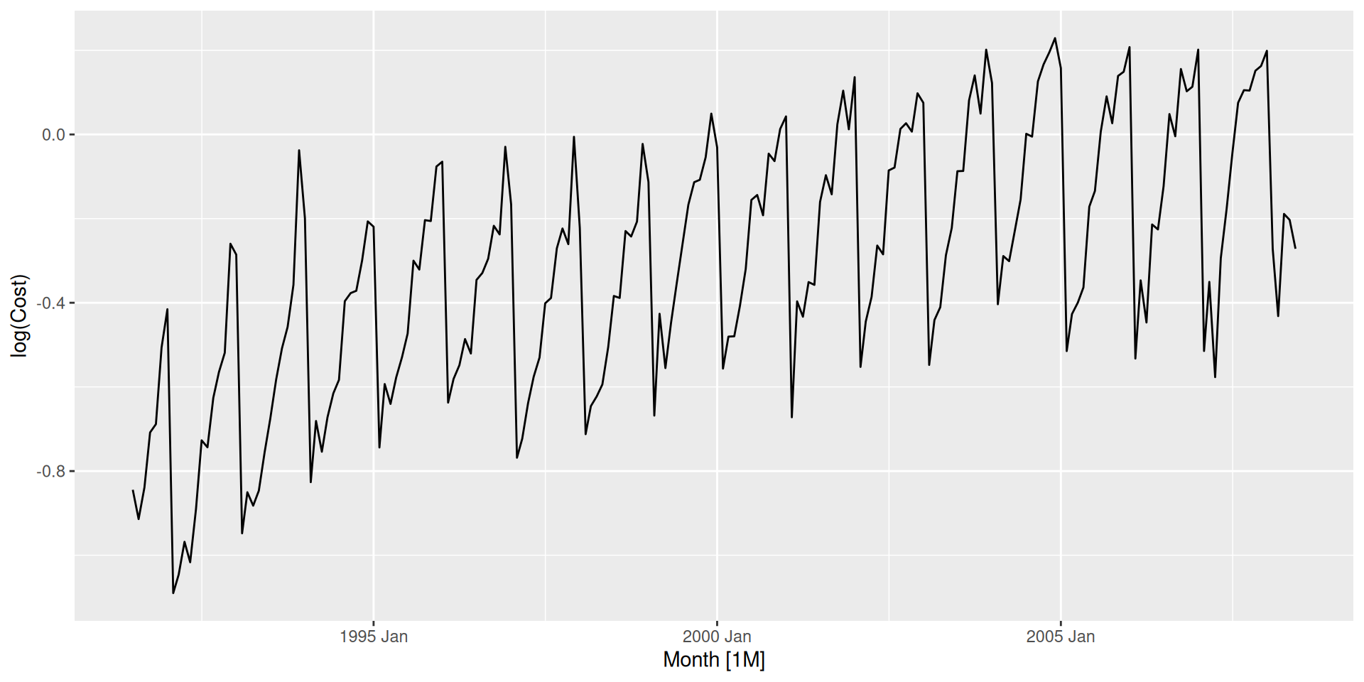
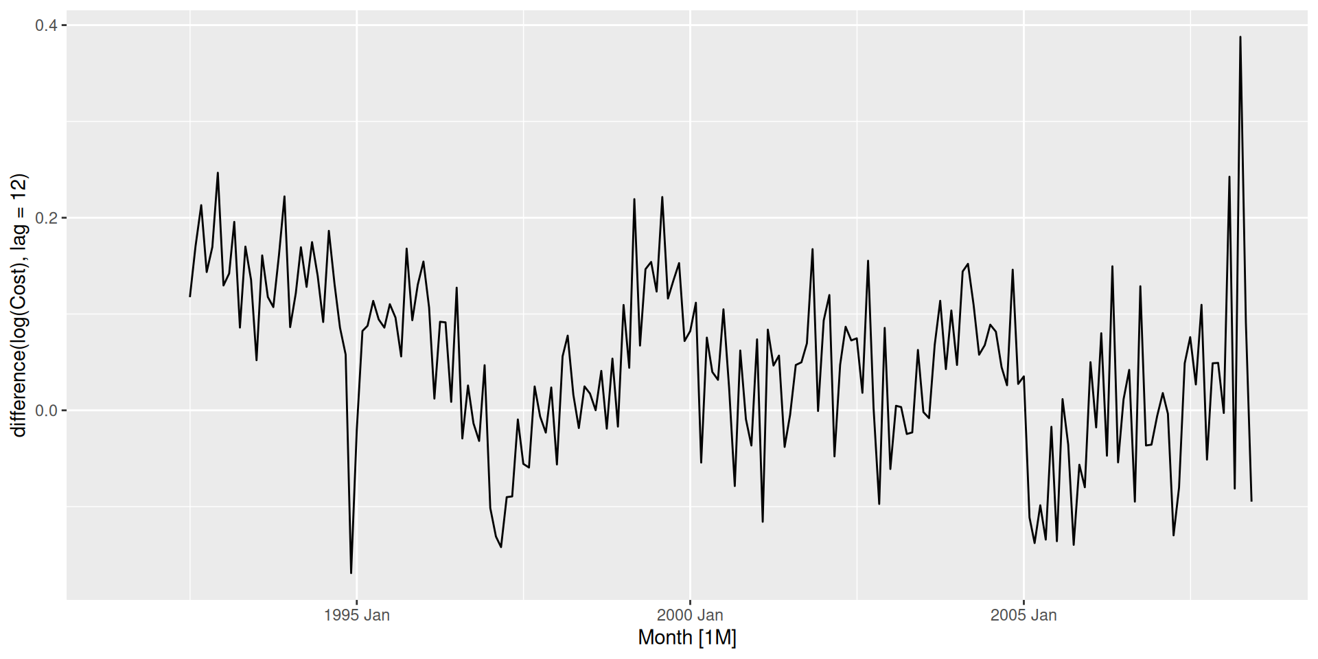
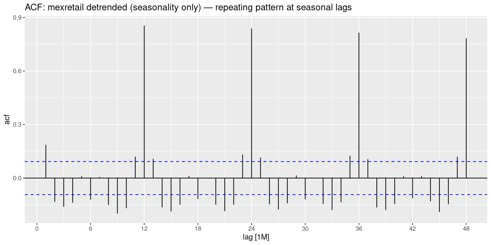
If the series has seasonality, we take a seasonal difference — the change relative to the same period in the previous cycle:
y'_t = y_t - y_{t-m}
where m is the seasonal period (m = 12 for monthly data, m = 4 for quarterly, …).
The backshift operator B provides a compact way to write differencing operations — and, as we will see next class, to write out full model equations cleanly.
It is defined simply as:
By_t = y_{t-1} ; B(By_t) = B^2 y_t = y_{t-2}
That is, applying B to a series shifts it back one period.
Recall the first difference:
y'_t = y_t - y_{t-1}
We can rewrite y_{t-1} = By_t, so:
y'_t = y_t - By_t = (1 - B)y_t
Recall:
y''_t = y_t - 2y_{t-1} + y_{t-2}
Using the backshift operator turns to:
y''_t = y_t - 2By_t + B^2 y_t = (1 - 2B + B^2)y_t
which gives a perfect square trinomial2
y''_t = (1-B)^2 y_t

The pattern generalizes naturally:
(1 - B)^d y_t
where d is the number of times we difference the series.
A seasonal difference shifts back m periods:
y_t - y_{t-m} = y_t - B^m y_t = (1 - B^m)y_t
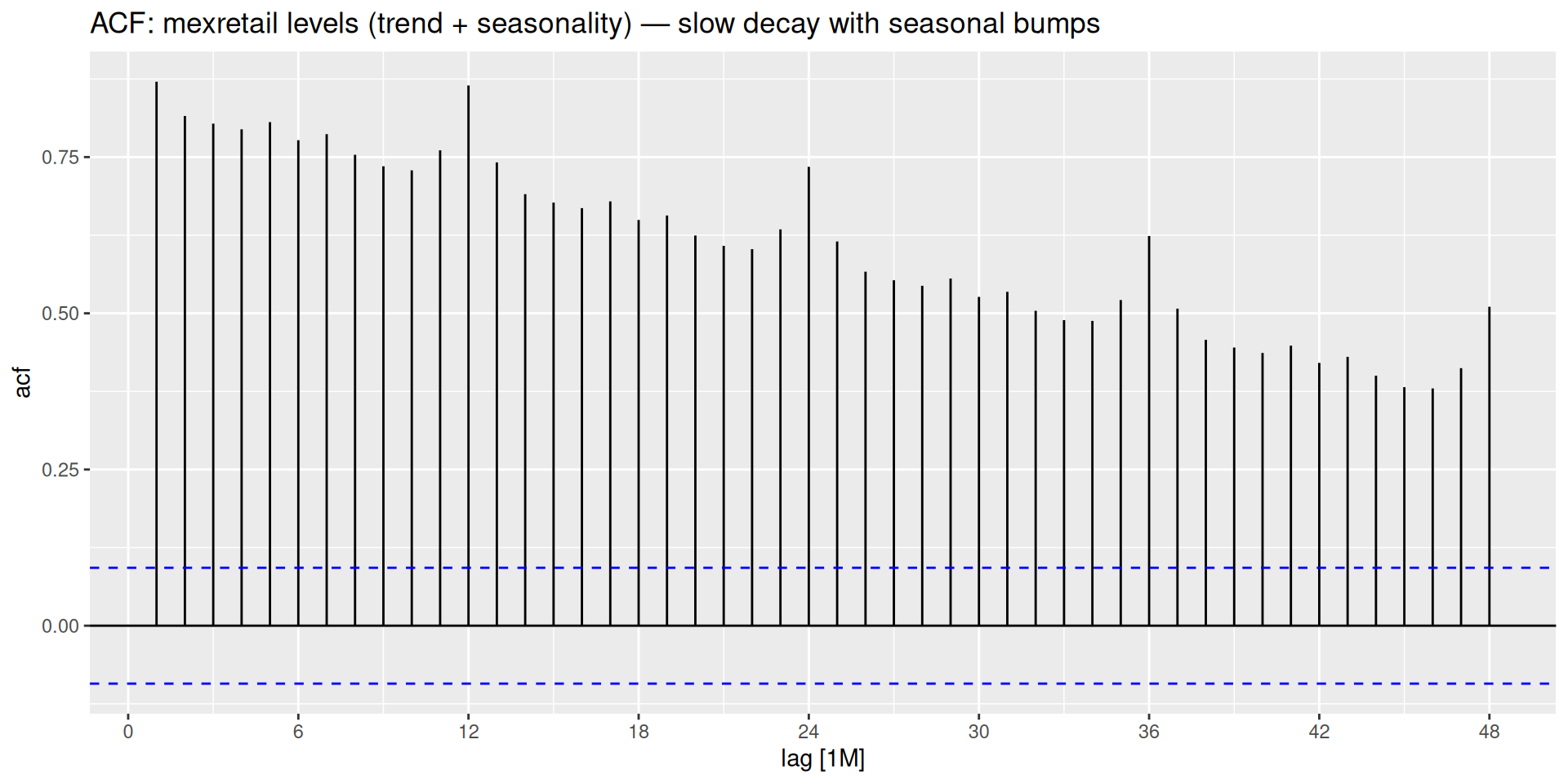
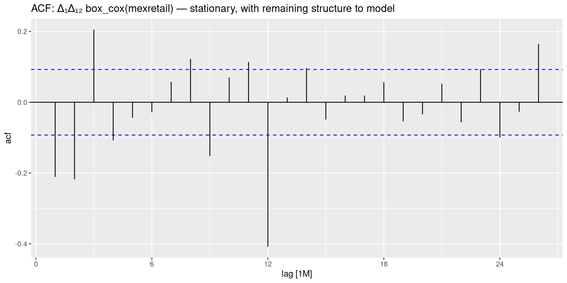
And when both are needed — as with mexretail — the two operators simply multiply:
(1-B)(1-B^m)y_t
which is exactly the expression we expanded by hand in the previous section.
| Operation | Backshift form |
|---|---|
| First difference | (1 - B)\,y_t |
| Second difference | (1 - B)^2\,y_t |
| d-th difference | (1 - B)^d\,y_t |
| Seasonal difference | (1 - B^m)\,y_t |
| Both together | (1 - B)^d(1 - B^m)\,y_t |
Order of differencing — revisited
Using backshift notation, it becomes trivial to see that the order doesn’t matter. Both orderings produce the same expression, since multiplication is commutative:
(1-B)(1-B^m)y_t = (1-B^m)(1-B)y_t
No algebra needed.
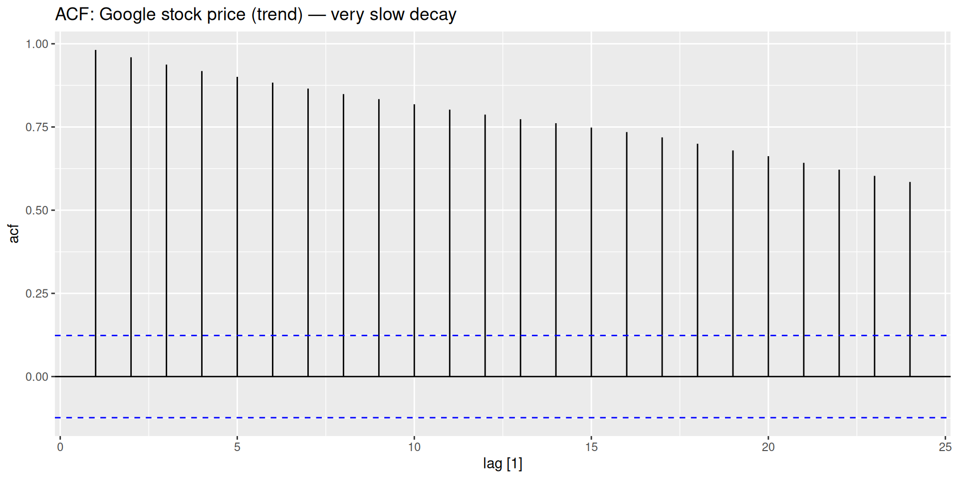
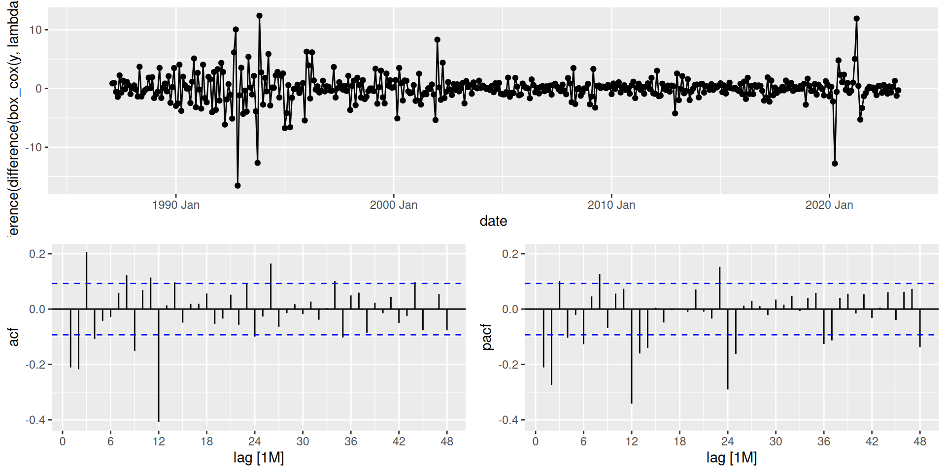
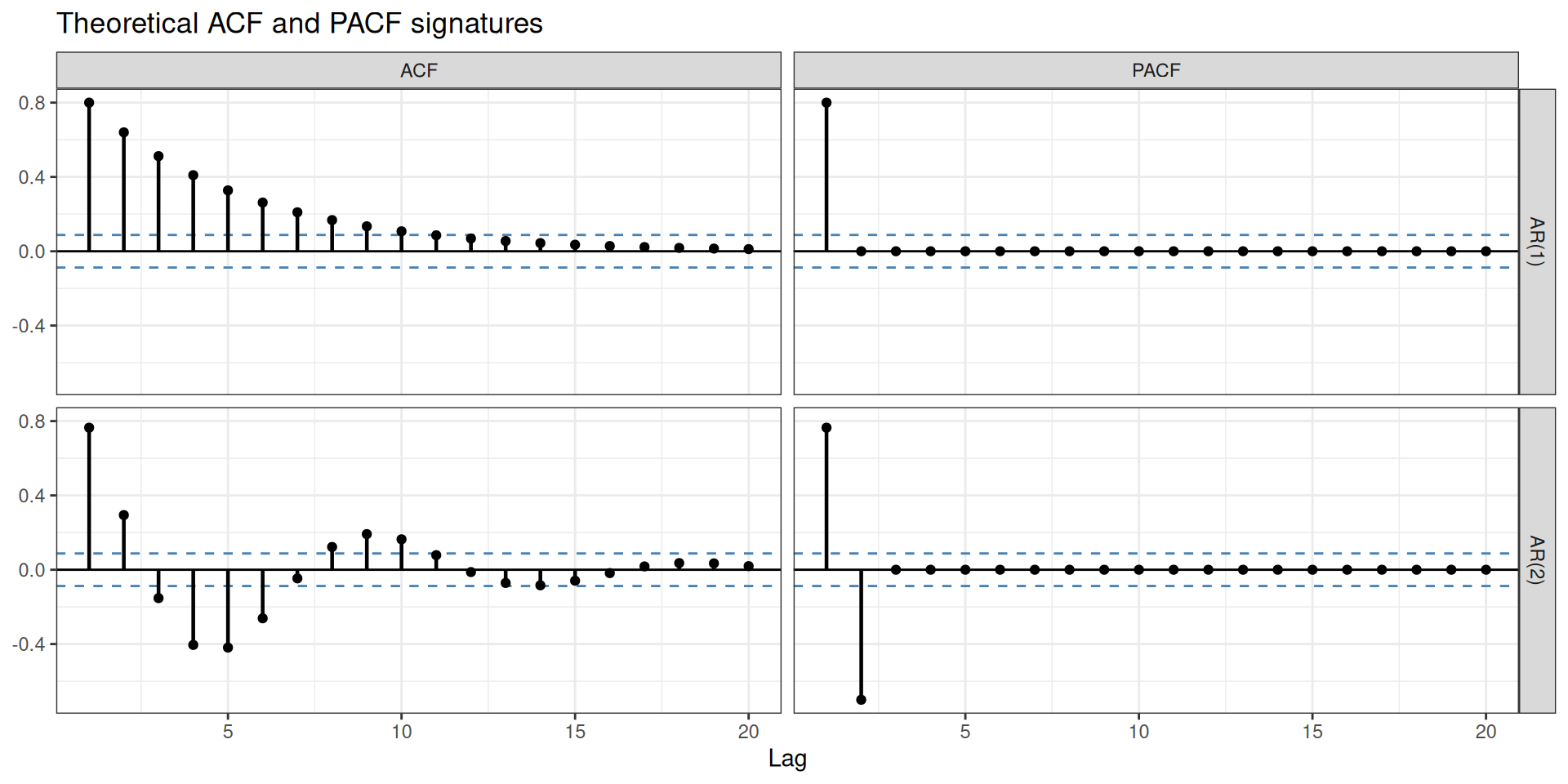
gg_tsdisplay() with plot_type = "partial" shows the time series, ACF, and PACF together — this is the standard diagnostic display for the rest of the module.
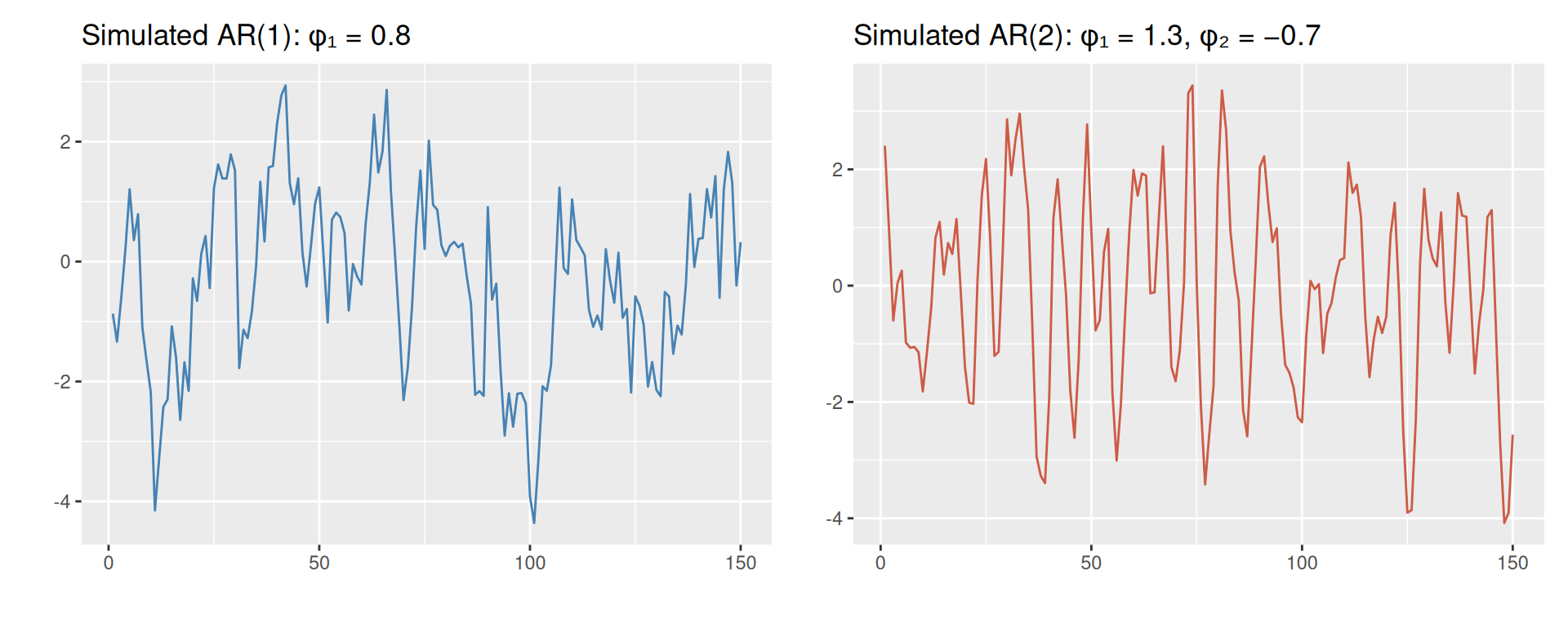
An autoregressive model of order p forecasts y_t as a weighted sum of its own past values:
y_t = c + \phi_1 y_{t-1} + \phi_2 y_{t-2} + \cdots + \phi_p y_{t-p} + \varepsilon_t
Signature in ACF/PACF
A moving average model of order q forecasts y_t as a weighted sum of past forecast errors:
y_t = c + \varepsilon_t + \theta_1 \varepsilon_{t-1} + \theta_2 \varepsilon_{t-2} + \cdots + \theta_q \varepsilon_{t-q}
MA models ≠ moving average smoothing
Do not confuse MA models with the moving average smoothing used in decomposition. Smoothing estimates the trend-cycle from past observed values. MA models use past errors to describe the correlation structure of the series.
Signature in ACF/PACF
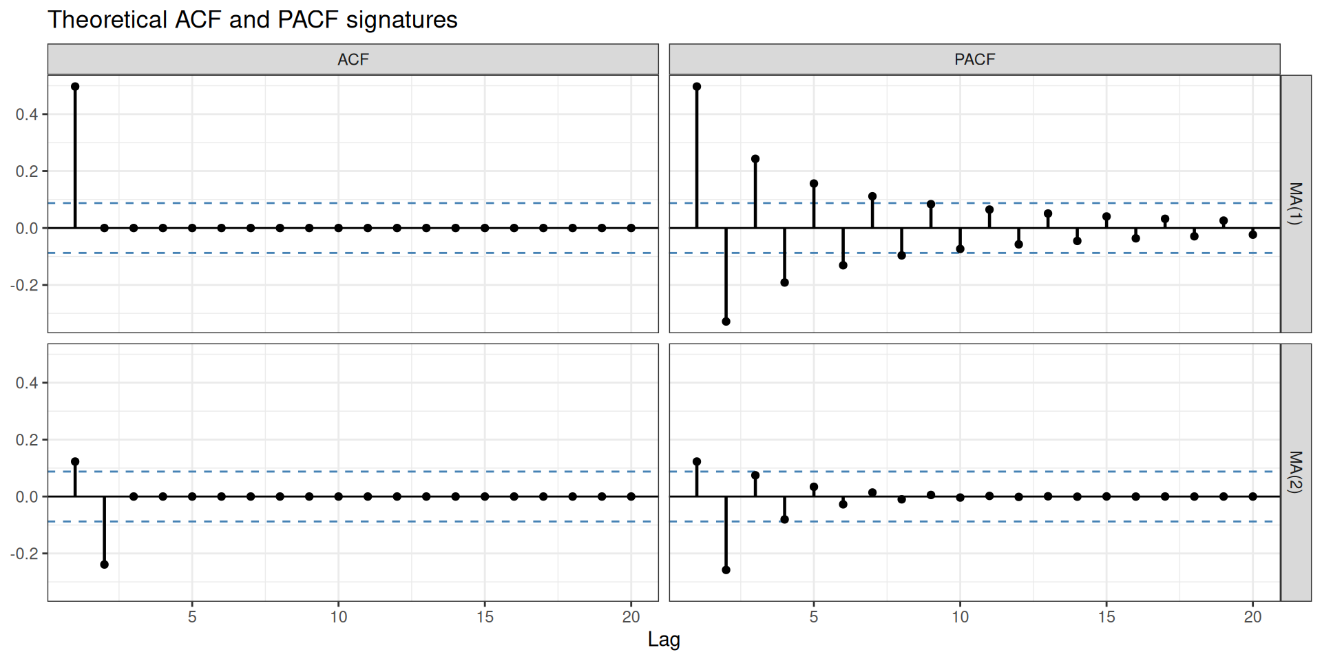
You cannot identify a model from the time plot alone
Now that you have seen AR and MA models: their time plots can look very similar to each other. The ACF and PACF are what distinguish them. This is fundamentally different from ETS, where the form of trend and seasonality in the time plot directly guides model selection — one of the key differences we will revisit when comparing these two families.
most commonly YoY (year-over-year), but remember there can be daily, weekly, or more seasonal patterns too.