Modular Forecasting: Mixing ETS and ARIMA

Data setup: mexretail

mexretail was first introduced in Module 1 — Time Series Decomposition and has been our running dataset throughout Module 2.

mexretail <- tq_get(
  "MEXSLRTTO01IXOBM",
  get = "economic.data",
  from = "1985-01-01"
) |>
  mutate(date = yearmonth(date)) |>
  rename(y = price) |>
  as_tsibble(index = date)

mexretail_train <- mexretail |> filter(year(date) <= 2019)
mexretail_test  <- mexretail |> filter(year(date) >  2019)

Where We Are

Module 2 has added two new model families to our toolkit. Together with decomposition_model(), they give us far more combinations than it might initially seem:

Approach	Decomposition	Trend-cycle	Seasonal
M1 baseline	STL	Drift	SNAIVE
STL + ETS	STL	ETS	SNAIVE
STL + ARIMA	STL	ARIMA	SNAIVE
STL + ETS + ARIMA	STL	ETS	ARIMA
STL + ARIMA + ETS	STL	ARIMA	ETS
ETS	—	ETS	ETS
SARIMA	—	ARIMA	ARIMA(P,D,Q)m

decomposition_model() is more flexible than it looked

In the previous sections, we always let STL handle the seasonal component implicitly — which defaults to SNAIVE. But decomposition_model() lets you specify a model for each component separately. This opens up the mixed combinations in the middle of the table, and that is exactly what we explore here.

Mixing ETS and ARIMA inside `decomposition_model()`

The structure

Recall the structure of decomposition_model():

decomposition_model(
  <decomposition method>,
  <model for season_adjust>,   # trend-cycle component
  <model for season_year>      # seasonal component (defaults to SNAIVE if omitted)
)

Each component has its own characteristics, and we can choose the best model for each one independently:

The constraint logic

Component	What it contains	What to suppress
`season_adjust`	trend + cycle + remainder	seasonality → `season("N")` / `PDQ(0,0,0)`
`season_year`	seasonal pattern only	trend → `trend("N")`

Defining the model specs

Rather than embedding the full decomposition_model() calls inside the mable, we define them as named objects first. This keeps the model comparison code clean and makes each specification easy to inspect and reuse.

baseline_spec <- decomposition_model(
  STL(log(y) ~
        trend(window = NULL) +
        season(window = "periodic"),
      robust = TRUE),
  RW(season_adjust ~ drift()),
  SNAIVE(season_year)
)

1: Module 1 baseline: STL + Drift + SNAIVE. Our benchmark — every model must beat this. See The Forecasting Workflow.

stl_ets_spec <- decomposition_model(
  STL(log(y) ~
        trend(window = NULL) +
        season(window = "periodic"),
      robust = TRUE),
  ETS(season_adjust ~ season("N"))
)

1: STL + ETS on the seasonally adjusted series; seasonal component defaults to SNAIVE. See Exponential Smoothing.
2: season("N") suppresses seasonality — STL already removed it from season_adjust.

stl_arima_spec <- decomposition_model(
  STL(log(y) ~
        trend(window = NULL) +
        season(window = "periodic"),
      robust = TRUE),
  ARIMA(season_adjust ~ PDQ(0, 0, 0))
)

1: STL + ARIMA on the seasonally adjusted series; seasonal component defaults to SNAIVE. See ARIMA Models.
2: PDQ(0,0,0) suppresses seasonal ARIMA terms — not needed on the seasonally adjusted series.

STL + ETS + ARIMA

ETS models the trend-cycle; ARIMA models the seasonal pattern:

stl_ets_arima_spec <- decomposition_model(
  STL(log(y) ~
        trend(window = NULL) +
        season(window = "periodic"),
      robust = TRUE),
  ETS(season_adjust ~ season("N")),
  ARIMA(season_year)
)

1: ETS with season("N") on the trend-cycle — no seasonality to model here.

STL + ARIMA + ETS

ARIMA models the trend-cycle; ETS models the seasonal pattern:

stl_arima_ets_spec <- decomposition_model(
  STL(log(y) ~
        trend(window = NULL) +
        season(window = "periodic"),
      robust = TRUE),
  ARIMA(season_adjust ~ PDQ(0, 0, 0)),
  ETS(season_year ~ trend("N"))
)

1: ARIMA with PDQ(0,0,0) on the trend-cycle — no seasonal ARIMA terms needed.
2: ETS with trend("N") on the seasonal component — the seasonal pattern has no trend.

Revisiting `mexretail`

Fitting all approaches

With the specs defined, the mable is straightforward to read — each row is a named approach:

mexretail_fit <- mexretail_train |>
  model(
    baseline      = baseline_spec,
    stl_ets       = stl_ets_spec,
    stl_arima     = stl_arima_spec,
    stl_ets_arima = stl_ets_arima_spec,
    stl_arima_ets = stl_arima_ets_spec,
    ets           = ETS(log(y)),
    sarima        = ARIMA(log(y),
                          stepwise      = FALSE,
                          approximation = FALSE)
  )

mexretail_fit

1: Full ETS without explicit decomposition — Holt-Winters handles everything internally. See Exponential Smoothing.
2: Full SARIMA without explicit decomposition. See ARIMA Models.

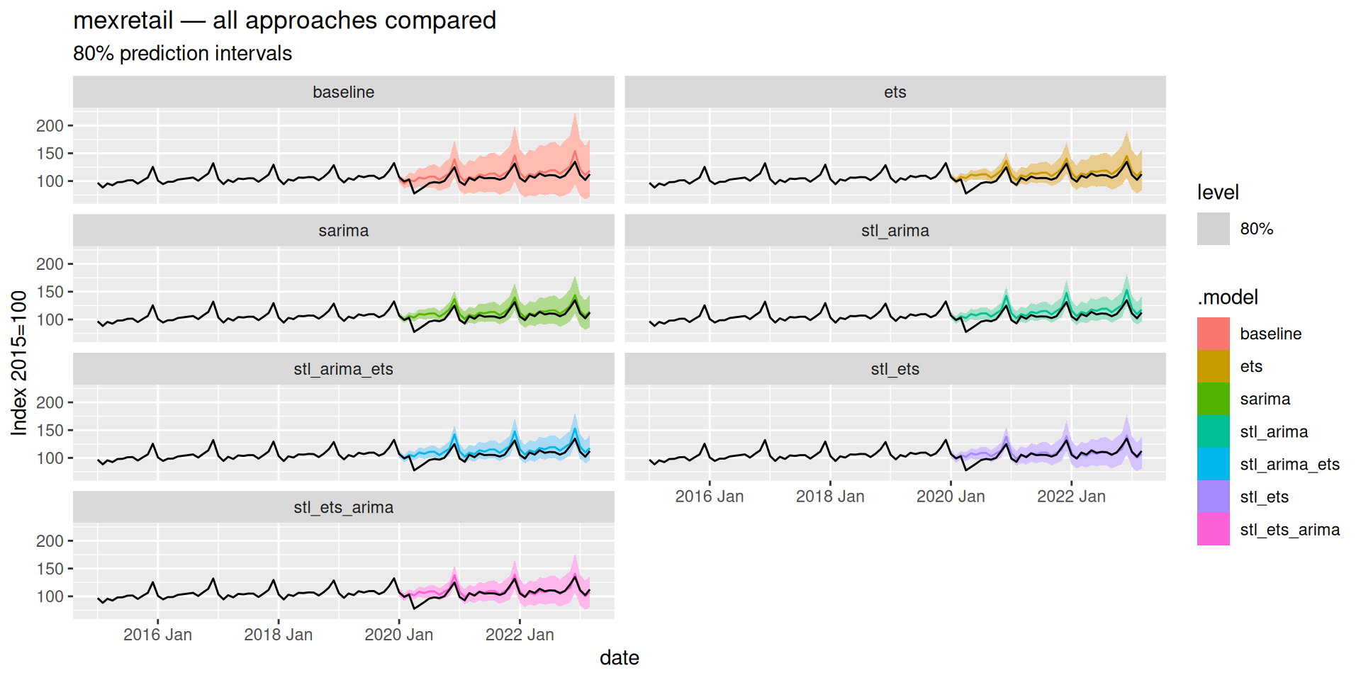
Forecasts

mexretail_fc <- mexretail_fit |>
  forecast(h = nrow(mexretail_test))

Accuracy on the test set

mexretail_accu <- mexretail_fc |>
  accuracy(mexretail) |>
  select(.model, RMSE, MAE, MAPE, MASE) |>
  arrange(RMSE)

mexretail_accu

Reading the table

A MASE below 1 means the model beats the SNAIVE benchmark. Check where baseline lands — that is the floor set in Module 1. Everything above it in this ranking is a genuine improvement.

A New Series: Australian Beer Production

Setup

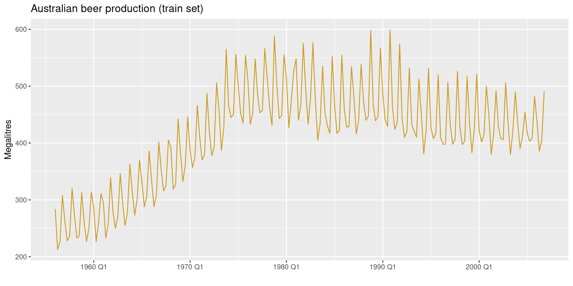
To check whether the rankings hold on a different series, we apply the same workflow to quarterly Australian beer production from fpp3:

beer_train <- aus_production |>
  rename(y = Beer) |>
  select(Quarter, y) |>
  filter(!is.na(y), year(Quarter) <= 2006)

beer_test <- aus_production |>
  rename(y = Beer) |>
  select(Quarter, y) |>
  filter(!is.na(y), year(Quarter) > 2006)

beer_full <- bind_rows(beer_train, beer_test)

1: We rename Beer to y — the same convention used for mexretail. This is what allows the specs defined above to be reused directly.

Reusing model specs across series

Because both mexretail and beer use log(y) as the response variable, the specs defined above apply to both series without any modification. The mable for beer will look identical to the one for mexretail — the only difference is the tsibble being piped in.

This is the payoff of two conventions working together: naming your response variable y, and defining specs outside the mable.

Fitting all approaches

beer_fit <- beer_train |>
  model(
    baseline      = baseline_spec,
    stl_ets       = stl_ets_spec,
    stl_arima     = stl_arima_spec,
    stl_ets_arima = stl_ets_arima_spec,
    stl_arima_ets = stl_arima_ets_spec,
    ets           = ETS(log(y)),
    sarima        = ARIMA(log(y), stepwise = FALSE, approximation = FALSE)
  )

beer_fit

Forecasts and accuracy

beer_fc <- beer_fit |>
  forecast(h = nrow(beer_test))

beer_accu <- beer_fc |>
  accuracy(beer_full) |>
  select(.model, RMSE, MAE, MAPE, MASE) |>
  arrange(RMSE)

beer_accu

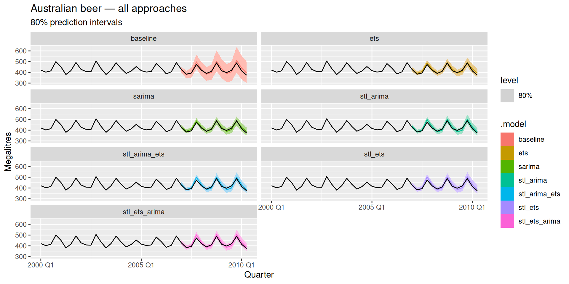
Does the winner change?

Compare the ranking here against mexretail. Does the same approach win on both series? What does that tell you about when mixed decomposition models add value — and when they don’t?

When to Use Which

Approach	Seasonal pattern	Outlier robustness	Best when…
STL + ETS	Flexible, can evolve	High	Trend smooth; seasonality stable
STL + ARIMA	Flexible, can evolve	High	Trend has autocorrelation structure
STL + ETS + ARIMA	Flexible, can evolve	High	Trend smooth; seasonal has autocorrelation
STL + ARIMA + ETS	Flexible, can evolve	High	Trend autocorrelated; seasonal is level-shifting
ETS	Fixed structure	Moderate	Short series; no explicit decomposition needed
SARIMA	Fixed structure	Lower	Compact model preferred; longer series

The guiding principle

No approach dominates universally. Always compare on a held-out test set. The mixed combinations (stl_ets_arima, stl_arima_ets) are not automatically better — they add flexibility but also complexity. Let the accuracy metrics decide.

Module 2 Wrap-Up

We started Module 2 with a single question: can we do better than Drift and SNAIVE?

We replaced Drift with ETS — adaptive smoothing that weights recent observations more heavily and handles a wide range of trend and seasonal patterns. (Exponential Smoothing)
We formalized stationarity, and learned to use Box-Cox transformations, differencing, and unit root tests to prepare a series for ARIMA modeling. (Stationarity & Differencing)
We built ARIMA models — combining differencing, AR, and MA terms into a unified framework, applied both inside STL and as a standalone seasonal model. (ARIMA Models)
Today, we discovered that decomposition_model() lets us mix ETS and ARIMA freely across components — and saw that naming specs separately keeps model comparison code clean and reusable across series.

What’s still missing?

All models in Module 2 are univariate — they only look at the history of the series itself, with no knowledge of the world outside: promotions, holidays, economic conditions, competitor behavior.

In Module 3, we give our models that external context by introducing regression with time series errors.

Modular Forecasting: Mixing ETS and ARIMA

Where We Are

Mixing ETS and ARIMA inside decomposition_model()

The structure

Defining the model specs

STL + ETS + ARIMA

STL + ARIMA + ETS

Revisiting mexretail

Fitting all approaches

Forecasts

Accuracy on the test set

A New Series: Australian Beer Production

Setup

Fitting all approaches

Forecasts and accuracy

When to Use Which

Module 2 Wrap-Up

Mixing ETS and ARIMA inside `decomposition_model()`

Revisiting `mexretail`