ARIMA Models

From AR/MA to ARIMA

In the previous topic we introduced the two basic building blocks for modeling the correlation structure of a stationary time series:

AR(p): forecast y_t using its own p past values.
MA(q): forecast y_t using q past forecast errors.

In practice, neither model alone is usually sufficient. Real series often show patterns that require both autoregressive and moving average components simultaneously. And most real series are also non-stationary — they have trend, seasonality, or both.

The natural next step

If we could combine AR and MA terms and relax the stationarity requirement by incorporating differencing directly into the model, we would have a single, unified framework for a very wide range of time series.

That framework is ARIMA.

The ARIMA Equation

ARIMA stands for AutoRegressive Integrated Moving Average. The “Integrated” part refers to the reverse operation of differencing: if we difference a series d times to make it stationary, the model is said to be integrated of order d.

A non-seasonal ARIMA model is written as ARIMA(p, d, q), where:

p — order of the autoregressive component (how many past values)
d — order of differencing (how many times we difference to achieve stationarity)
q — order of the moving average component (how many past errors)

The model equation, written on the differenced series y'_t, is:

y'_t = c + \phi_1 y'_{t-1} + \cdots + \phi_p y'_{t-p} + \theta_1 \varepsilon_{t-1} + \cdots + \theta_q \varepsilon_{t-q} + \varepsilon_t

where y'_t denotes the d-times differenced series and \varepsilon_t is white noise.

Backshift Notation

Recall from the previous topic that the backshift operator B satisfies By_t = y_{t-1}, and that d-th order differencing can be written as (1-B)^d y_t.

Using this notation, we can write the AR and MA components compactly as well:

AR component: \phi_1 y_{t-1} + \phi_2 y_{t-2} + \cdots + \phi_p y_{t-p} = \phi(B)\,y_t

where \phi(B) = \phi_1 B + \phi_2 B^2 + \cdots + \phi_p B^p.

MA component: \theta_1 \varepsilon_{t-1} + \theta_2 \varepsilon_{t-2} + \cdots + \theta_q \varepsilon_{t-q} = \theta(B)\,\varepsilon_t

where \theta(B) = \theta_1 B + \theta_2 B^2 + \cdots + \theta_q B^q.

Full ARIMA(p, d, q) in backshift notation:

\underbrace{(1 - \phi_1 B - \cdots - \phi_p B^p)}_{\text{AR}(p)} \underbrace{(1-B)^d}_{\text{differencing}} y_t = c + \underbrace{(1 + \theta_1 B + \cdots + \theta_q B^q)}_{\text{MA}(q)} \varepsilon_t

This compact form shows clearly how the three components interact. The differencing operator (1-B)^d is applied first, and the AR and MA operators act on the resulting stationary series.

Special Cases

Several models we have already encountered are special cases of the ARIMA family:

Model	ARIMA specification
White noise	ARIMA(0, 0, 0) without constant
Random walk	ARIMA(0, 1, 0) without constant
Random walk with drift	ARIMA(0, 1, 0) with constant
AR(p)	ARIMA(p, 0, 0)
MA(q)	ARIMA(0, 0, q)

Effect of c and d on long-run forecasts

The constant c and the differencing order d interact to determine the long-run behavior of ARIMA forecasts:

d = 0, c = 0: forecasts go to zero.
d = 0, c \neq 0: forecasts go to the mean of the series.
d = 1, c = 0: forecasts approach a non-zero constant.
d = 1, c \neq 0: forecasts follow a straight line.
d = 2, c \neq 0: forecasts follow a quadratic trend.

Higher values of d also produce wider prediction intervals that grow faster.

ARIMA in R

Choosing the Orders

Selecting the right ARIMA order involves three decisions:

Choose d — determine how many differences are needed using the stationarity protocol from the previous topic: Box-Cox / log transformation to stabilize variance, unitroot_nsdiffs() for seasonal differencing (if any), then unitroot_ndiffs() on the differenced series.
Choose p or q — read the ACF and PACF of the (differenced, stationary) series:
- PACF cuts off after lag p → AR(p) component.
- ACF cuts off after lag q → MA(q) component.
- Both decay gradually → mixed ARMA, try several combinations.
Compare candidates using information criteria (see Model Selection).

ACF/PACF reading is a starting point, not a definitive answer

Real data rarely produces textbook-perfect ACF/PACF shapes. Use the plots to narrow down candidate models, then compare them formally with AIC_c.

Manual and Automatic Specification

In fable, ARIMA models are specified inside model() using the ARIMA() function. The order is controlled with pdq() for non-seasonal terms and PDQ() for seasonal terms. When pdq() is left unspecified, fable searches for the best order automatically.

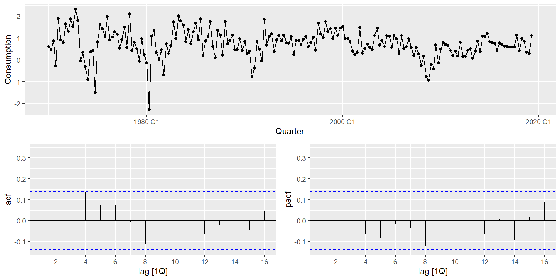
The series appears stationary (d = 0). The PACF shows significant spikes at lags 1–3, suggesting AR(3). We can fit this manually, compare it against automatic selection strategies, and let AIC_c arbitrate — all within a single mable:

us_change_fit <- us_change |>
  model(
    manual     = ARIMA(Consumption ~ pdq(3, 0, 0) + PDQ(0, 0, 0)),
    auto       = ARIMA(Consumption ~ PDQ(0, 0, 0)),
    semi_auto  = ARIMA(Consumption ~ pdq(1:3, 0, 0:2) + PDQ(0, 0, 0)),
    exhaustive = ARIMA(Consumption ~ PDQ(0, 0, 0),
                       stepwise      = FALSE,
                       approximation = FALSE)
  )

glance(us_change_fit) |>
  arrange(AICc) |>
  select(.model, AIC, AICc, BIC)

1: Manual specification using pdq(). PDQ(0,0,0) explicitly forces a non-seasonal model.
2: Leaving pdq() unspecified triggers automatic stepwise order selection.
3: Evaluates all combinations of p \in \{1,2,3\} and q \in \{0,1,2\}, returns the lowest AIC_c.
4: stepwise = FALSE explores all combinations rather than navigating step by step.
5: approximation = FALSE uses exact likelihood. More accurate but slower on long series.

How does automatic selection work?

fable implements a stepwise search algorithm (Hyndman & Khandakar, 2008) that:

Determines d using unit root tests.
Starts from a simple model and navigates through the order space by comparing AIC_c values.
Stops when no neighboring model improves AIC_c.

Important: this is a heuristic search — it does not evaluate all possible combinations. It is fast and usually good, but not guaranteed to find the global optimum.

For exploratory work, automatic selection is fine. For a final model, use stepwise = FALSE, approximation = FALSE and compare the result with your manually identified candidate.

How much slower is exhaustive search?

stepwise = FALSE, approximation = FALSE triggers a full search over all candidate models using exact likelihood. The difference in runtime can be dramatic:

tictoc::tic("auto")
us_change |>
  model(ARIMA(Consumption ~ PDQ(0, 0, 0)))

tictoc::toc()

auto: 0.24 sec elapsed

tictoc::tic("exhaustive")
us_change |>
  model(ARIMA(Consumption ~ PDQ(0, 0, 0),
              stepwise      = FALSE,
              approximation = FALSE))

tictoc::toc()

exhaustive: 1.06 sec elapsed

Times will vary by hardware, but the relative difference is what matters. On longer series like mexretail (480+ monthly observations with seasonal structure), the gap is even more pronounced — which is why freeze is recommended for documents containing exhaustive ARIMA searches.

Model Selection

When comparing candidate ARIMA models, we use three related criteria:

AIC — Akaike Information Criterion
AIC_c — AIC corrected for small sample sizes
BIC — Bayesian Information Criterion (also known as Schwarz criterion)

\text{AIC} = -2\log(L) + 2(p + q + k + 1)

\text{AIC}_c = \text{AIC} + \frac{2(p + q + k + 1)(p + q + k + 2)}{T - p - q - k - 2}

\text{BIC} = \text{AIC} + [\log(T) - 2](p + q + k + 1)

where k = 1 if the model includes a constant, k = 0 otherwise. Lower is better for all three. The preferred criterion is AIC_c — it converges to AIC as T grows, but is more conservative with small samples.

Information criteria require the same scale

Information criteria are only comparable across models fitted to identical data — same transformation, same differencing order. You cannot compare AIC_c of an ARIMA fitted to \log(y_t) vs. one fitted to y_t, or ARIMA(1,1,1) vs. ARIMA(1,0,1). When models differ in d, use forecast accuracy on a test set instead.

Box-Jenkins Methodology

ARIMA model building follows an iterative procedure known as the Box-Jenkins methodology:

Plot the data. Identify unusual observations, structural breaks, outliers.
Stabilize the variance if needed — apply a log or Box-Cox transformation.
Determine d — use unitroot_nsdiffs() and unitroot_ndiffs().
Examine ACF and PACF of the stationary series to identify candidate orders p and q.
Fit candidate models and compare using AIC_c.
Check residuals — ACF of residuals and Ljung-Box test. If not white noise, refine.
Forecast once residuals pass diagnostic checks.

It’s iterative

The Box-Jenkins procedure is a cycle, not a checklist. It is normal to go through steps 4–6 two or three times before settling on a model.

Residual Diagnostics

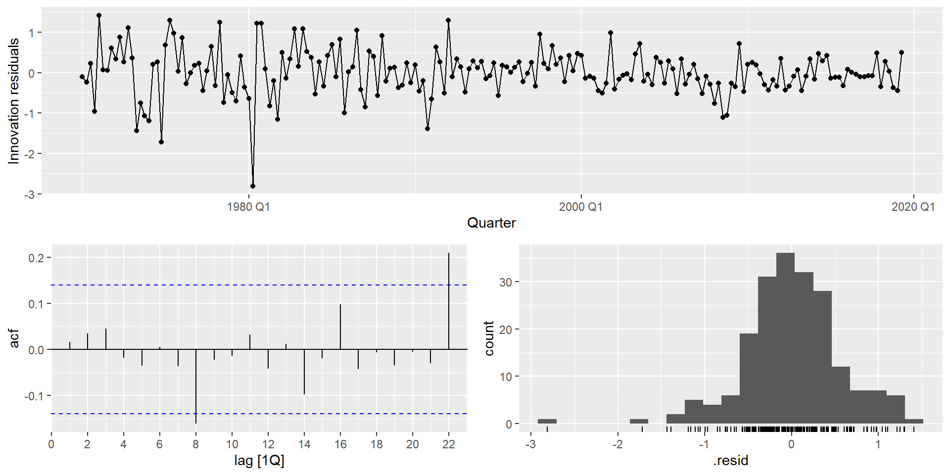
We have already used the Ljung-Box test to check residuals from benchmark models. When applying it to ARIMA models, there is one important adjustment: you must account for the degrees of freedom consumed by the estimated AR and MA parameters.

us_change_fit |>
  select(manual) |>
  gg_tsresiduals()

us_change_fit |>
  select(manual) |>
  augment() |>
  features(.innov, ljung_box,
           lag = 10,
           dof = us_change_fit |>
                   select(manual) |>
                   coefficients() |>
                   filter(str_detect(term, "^ar|^ma")) |>
                   nrow())

1: dof is computed dynamically as the number of estimated AR and MA coefficients, so it always matches the fitted model regardless of order.

Forecasting

Once the model passes residual diagnostics, forecasting uses the same forecast() workflow as all other fable models:

us_change_fit |>
  select(manual) |>
  forecast(h = 10) |>
  autoplot(us_change |> filter(year(Quarter) >= 2005)) +
  labs(
    title = "US consumption — ARIMA(3,0,0) forecast",
    y = "% change"
  )

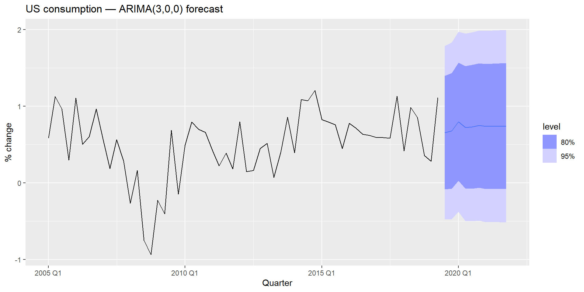
Prediction intervals

ARIMA prediction intervals are derived analytically from the model’s MA representation. Their width grows with the forecast horizon, and grows faster as d increases — a direct consequence of accumulated uncertainty from differencing. For a random walk (d = 1), intervals widen at rate \sqrt{h}; for d = 2, they widen even faster.

Seasonal ARIMA

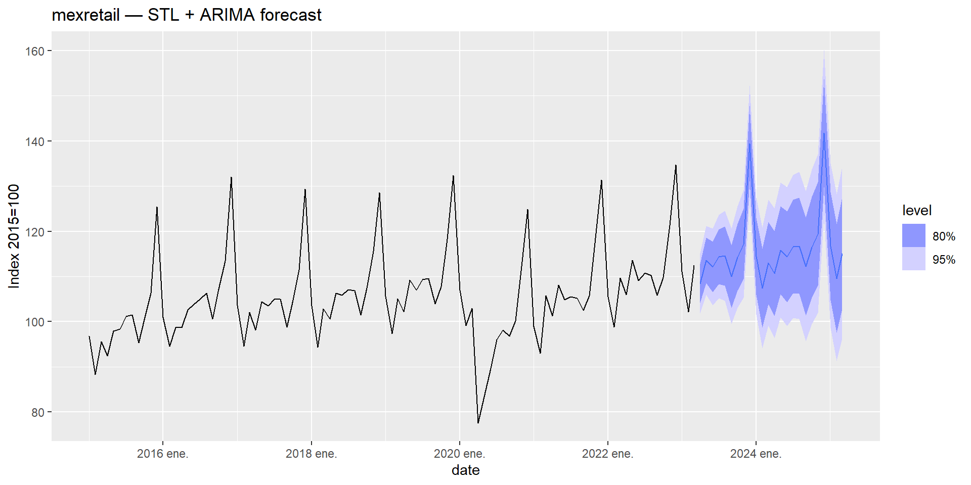
STL + ARIMA

mexretail is a monthly series with strong trend and seasonality. We already know how to handle it with STL decomposition. In Module 1 we combined STL with SNAIVE; in Module 2 we replaced SNAIVE with ETS. The natural next step is to replace it with ARIMA.

The idea is the same: use STL to handle the seasonal pattern, and let ARIMA model the trend-cycle on the seasonally adjusted series.

mexretail_fit_stl_arima <- mexretail |>
  model(
    stl_arima = decomposition_model(
      STL(box_cox(y, lambda) ~
            season(window = "periodic"),
          robust = TRUE),
      ARIMA(season_adjust ~ PDQ(0,0,0))
    )
  )

report(mexretail_fit_stl_arima)

1: decomposition_model() combines a decomposition method with a model for one or more of its components.
2: STL decomposes the Box-Cox-transformed series. The seasonal component is handled implicitly by the decomposition.
3: ARIMA(season_adjust) fits an ARIMA model automatically to the seasonally adjusted component. The seasonal part is re-added when generating forecasts.

Series: y 
Model: STL decomposition model 
Transformation: box_cox(y, lambda) 
Combination: season_adjust + season_year

========================================

Series: season_adjust 
Model: ARIMA(0,1,1) w/ drift 

Coefficients:
          ma1  constant
      -0.4500    0.1007
s.e.   0.0433    0.0491

sigma^2 estimated as 3.553:  log likelihood=-914.69
AIC=1835.38   AICc=1835.43   BIC=1847.68

Series: season_year 
Model: SNAIVE 

sigma^2: 0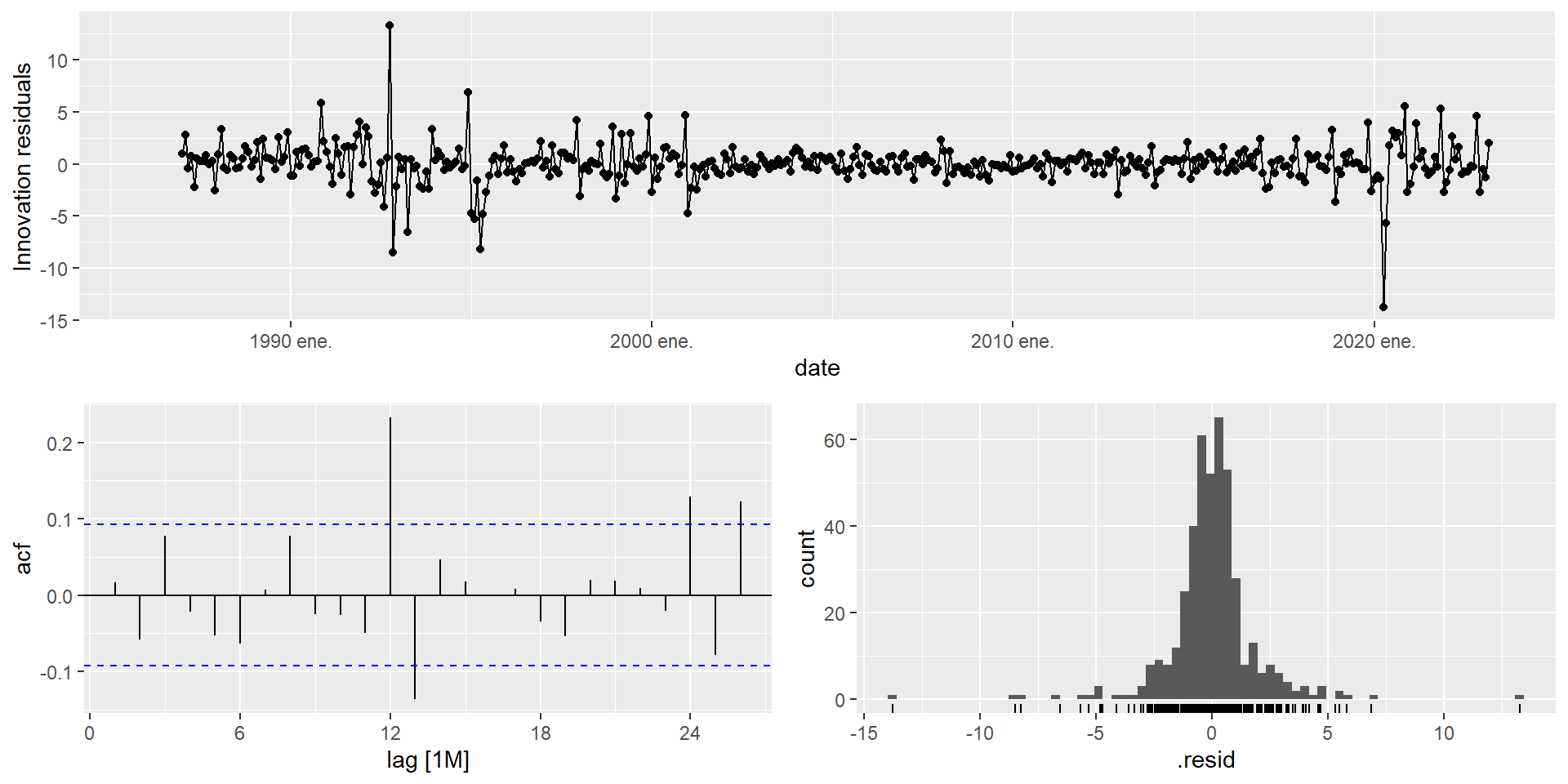

mexretail_fit_stl_arima |> gg_tsresiduals()

mexretail_fit_stl_arima |>
  forecast(h = 24) |>
  autoplot(mexretail |> filter(year(date) >= 2015)) +
  labs(
    title = "mexretail — STL + ARIMA forecast",
    y = "Index 2015=100"
  )

SARIMA

STL + ARIMA is a two-stage approach: decompose first, then model. An alternative is to handle seasonality within a single ARIMA model by adding seasonal AR and MA terms. This is a Seasonal ARIMA model, written as:

\text{ARIMA}\underbrace{(p,\,d,\,q)}_{\text{non-seasonal}}\underbrace{(P,\,D,\,Q)_{m}}_{\text{seasonal}}

where m is the seasonal period (m = 12 for monthly data).

The full model in backshift notation is:

\underbrace{\Phi(B^m)}_{\text{seasonal AR}} \underbrace{\phi(B)}_{\text{non-seasonal AR}} \underbrace{(1-B^m)^D (1-B)^d}_{\text{differencing}} y_t = c + \underbrace{\Theta(B^m)}_{\text{seasonal MA}} \underbrace{\theta(B)}_{\text{non-seasonal MA}} \varepsilon_t

Reading ACF/PACF for Seasonal Orders

The non-seasonal orders (p, q) are read from the first few lags of the ACF/PACF, as before. The seasonal orders (P, Q) are read from the seasonal lags (m, 2m, 3m, …):

Pattern at seasonal lags	Suggested component
PACF spikes cut off after lag Pm	Seasonal AR(P)
ACF spikes cut off after lag Qm	Seasonal MA(Q)
Both decay gradually	Mixed seasonal ARMA

Focus on the seasonal lags separately from the non-seasonal lags. Use lag_max = 3m or 4m to make the seasonal structure clearly visible.

SARIMA for `mexretail`

The stationarity protocol for mexretail established that we need D = 1 and d = 1 applied to the Box-Cox-transformed series. Let’s inspect the ACF/PACF to choose p, q, P, Q:

mexretail |>
  gg_tsdisplay(
    difference(box_cox(y, lambda), 12) |> difference(1),
    plot_type = "partial",
    lag_max   = 48
  )

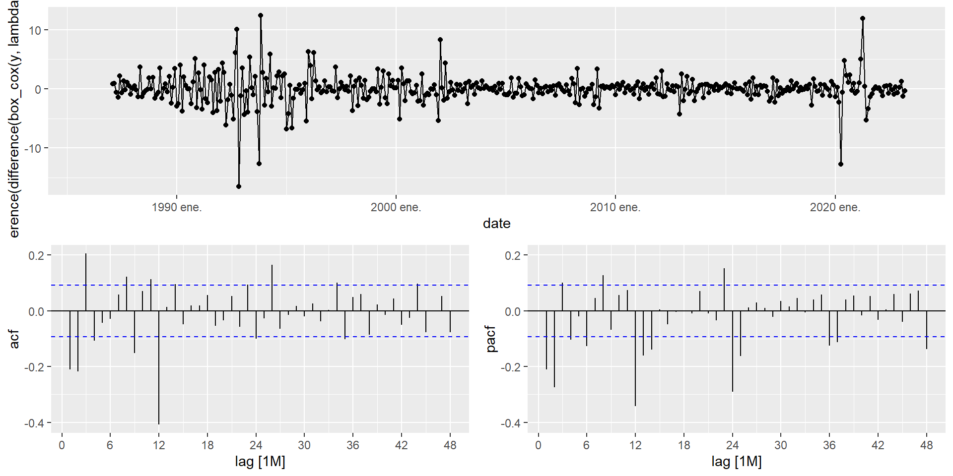
Reading the plot

Non-seasonal lags (1–11):
- ACF: spike at lag 1, and up to lag 4 → try q = 1 up to q = 4.
- PACF: spikes at lags 1 and 2, borderline at lag 3 → try p = 2 or p = 3.
Seasonal lags (12, 24, 36, 48):
- ACF: spike at lag 12, barely at lag 24 → try Q = 1 or Q = 2.
- PACF: spikes at lags 12, 24, and slightly at 36 and 48 → try P = 2, P = 3, or even P = 4.

When ACF/PACF suggest large orders, start simple

A strict reading of the ACF/PACF above could justify orders as large as AR(3), MA(4), SAR(4), SMA(2) — a model with over a dozen parameters. In practice, this is rarely a good starting point: high-order models are harder to estimate, more prone to overfitting, and — if specified manually — can fail to converge or return non-invertible roots altogether.

A better strategy: start with a parsimonious candidate like \text{ARIMA}(0,1,1)(0,1,1)_{12} or \text{ARIMA}(1,1,1)(1,1,1)_{12}, fit a few of the larger candidates suggested by the plots, and let AIC_c arbitrate. You will often find that the simpler model performs comparably or better — and it will always be more stable.

mexretail_fit_sarima <- mexretail |>
  model(
    sarima_011_110 = ARIMA(box_cox(y, lambda) ~
                             pdq(0, 1, 1) + PDQ(1, 1, 0)),
    sarima_011_011 = ARIMA(box_cox(y, lambda) ~
                             pdq(0, 1, 1) + PDQ(0, 1, 1)),
    sarima_auto    = ARIMA(box_cox(y, lambda),
                           stepwise      = FALSE,
                           approximation = FALSE)
  )

glance(mexretail_fit_sarima) |>
  arrange(AICc) |>
  select(.model, AIC, AICc, BIC)

1: First candidate from ACF/PACF: non-seasonal MA(1), seasonal AR(1).
2: Second candidate: non-seasonal MA(1), seasonal MA(1) — a very common structure for monthly economic data.
3: Exhaustive automatic search for comparison.

mexretail_fit_sarima |>
  select(sarima_auto) |>
  report()

Series: y 
Model: ARIMA(3,0,1)(0,1,2)[12] w/ drift 
Transformation: box_cox(y, lambda) 

Coefficients:
         ar1     ar2     ar3     ma1     sma1     sma2  constant
      0.2930  0.3114  0.3143  0.3671  -0.6877  -0.0956    0.0931
s.e.  0.1848  0.1454  0.0521  0.1975   0.0526   0.0534    0.0274

sigma^2 estimated as 3.303:  log likelihood=-879.31
AIC=1774.62   AICc=1774.95   BIC=1807.22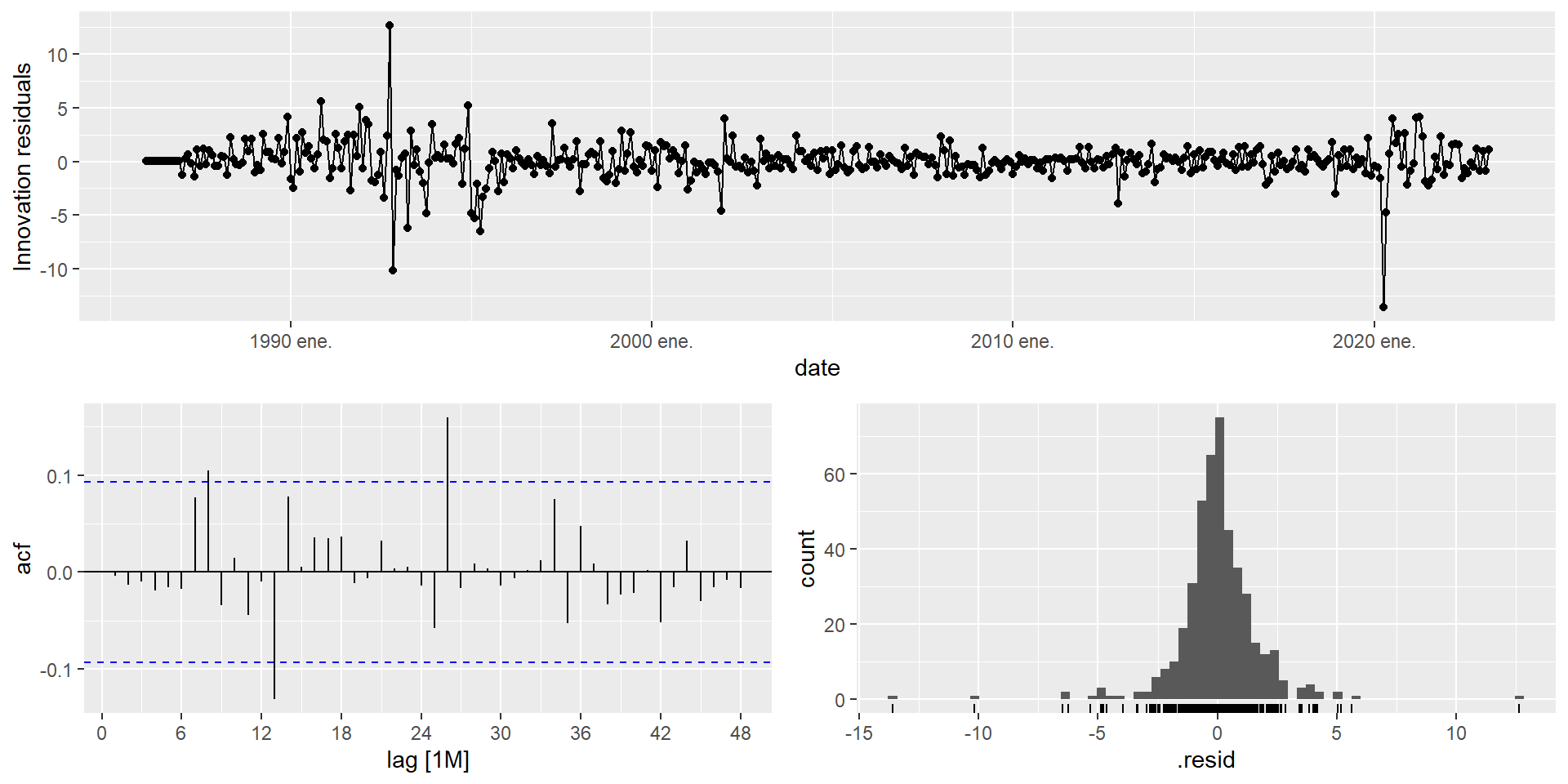

mexretail_fit_sarima |>
  select(sarima_auto) |>
  gg_tsresiduals(lag_max = 48)

mexretail_fit_sarima |>
  select(sarima_auto) |>
  augment() |>
  features(.innov, ljung_box,
           lag = 24,
           dof = mexretail_fit_sarima |>
                   select(sarima_auto) |>
                   coefficients() |>
                   filter(str_detect(term, "^ar|^ma|^sar|^sma")) |>
                   nrow())

1: dof is computed dynamically as p + q + P + Q for the fitted model, so it always reflects the actual order selected by the exhaustive search.

STL + ARIMA vs. SARIMA

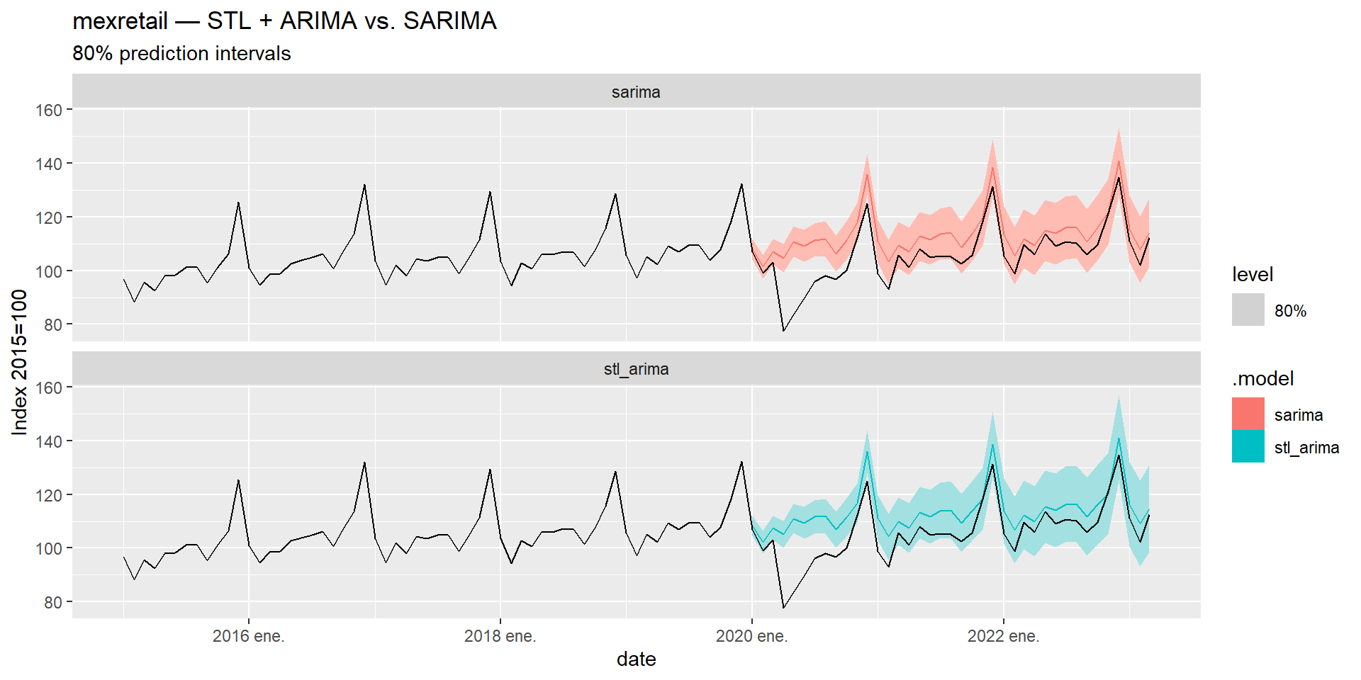
Comparing Both Strategies

Both approaches are valid for seasonal series. Let’s compare them on mexretail using a train/test split:

mexretail_train <- mexretail |> filter(year(date) <= 2019)
mexretail_test  <- mexretail |> filter(year(date) >  2019)

mexretail_fit <- mexretail_train |>
  model(
    stl_arima = decomposition_model(
      STL(box_cox(y, lambda) ~
            trend(window = NULL) +
            season(window = "periodic"),
          robust = TRUE),
      ARIMA(season_adjust)
    ),
    sarima = ARIMA(box_cox(y, lambda),
                   stepwise      = FALSE,
                   approximation = FALSE)
  )

mexretail_fit |>
  forecast(h = nrow(mexretail_test)) |>
  accuracy(mexretail) |>
  select(.model, RMSE, MAE, MAPE, MASE) |>
  arrange(RMSE)

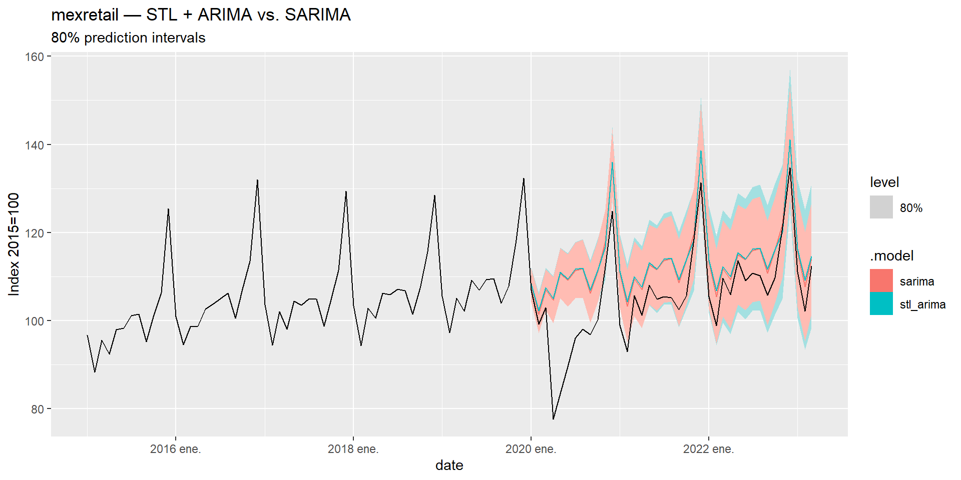
When to use which

	STL + ARIMA	SARIMA
Seasonal pattern	Flexible — can change over time	Fixed structure
Outlier robustness	High (with `robust = TRUE`)	Lower
Interpretability	Decomposition is visible	Single compact model
Multiple seasonality	Handles it naturally	Difficult
Parsimony	Two models in sequence	One unified model

Neither approach dominates universally. Let the data and the accuracy metrics guide the choice.

ARIMA Models

ARIMA Models

From AR/MA to ARIMA

The ARIMA Equation

Backshift Notation

Special Cases

ARIMA in R

Choosing the Orders

Manual and Automatic Specification

Model Selection

Box-Jenkins Methodology

Residual Diagnostics

Forecasting

Seasonal ARIMA

STL + ARIMA

SARIMA

Reading ACF/PACF for Seasonal Orders

SARIMA for mexretail

STL + ARIMA vs. SARIMA

Comparing Both Strategies

SARIMA for `mexretail`