Time Series Decomposition

pbenavides

TS Features & Patterns

All these time series have different shapes, patterns, and so on. When modeling them, we need to take these characteristics into account. We seek to understand the underlying patterns in the data to make better forecasts.

TS Patterns

Time series can have distinct patterns:

• Trend: A long-term increase/decrease in the data.

• Seasonal: Fluctuations in the time series with a fixed and known period¹.

• Cycles: More commonly known as “Business cycles”, refer to rises and falls that are not of a fixed frequency².

• Changes in variability: Changes in the spread of the data over time, i. e., an increase/decrease in the variance as the level of the series increases/decreases.

Components of a Time Series

A time series can be decomposed into the following components:

• Seasonal component (S): The repeating short-term cycle in the series.

• Trend-cycle component (T): The long-term progression of the series.

• Residual component (R): The residuals or “noise” left after removing the seasonal and trend-cycle components.

Mathematical Transformations

Transformations are used to stabilize the variance of a time series, making it easier to model and forecast. They can help to make the patterns in the data more apparent.

Log transformations

• Series in levels
• Log

Transformations and adjustments help us simplify the patterns in our data, and can improve our forecasts’ accuracy.

• Log transformations are often useful when the data presents an increasing/decreasing variation with the level of the series.

• Log transformations are very interpretable: changes in a log value are percent changes on the original scale.

Box-Cox transformations

\[ w_t= \begin{cases}\log \left(y_t\right) & \text { if } \lambda=0 \\ \left(\operatorname{sign}\left(y_t\right)\left|y_t\right|^\lambda-1\right) / \lambda & \text { otherwise }\end{cases} \]

In a Box-Cox transformation, the log is always a natural logarithm. The other case is just a power transformation with scaling.

What happens when \(\lambda = 1\)?

You should choose a value of \(\lambda\) that makes the size of the seasonal variation the same throughout the series.

How can we choose the value of \(\lambda\)?

How can we choose the value of \(\lambda\)?

We can use the guerrero feature to choose an optimal lambda.

aus_production |> 
  features(Gas, features = guerrero)

# A tibble: 1 × 1
  lambda_guerrero
            <dbl>
1           0.110

Time Series Adjustments

Calendar adjustments

• Closing price and volume
• Monthly aggregation
• Monthly total and mean and volume

google_month <- google |> 
  index_by(month = yearmonth(date)) |> 
  summarise(
    trading_days = n(),
    monthly_volume = sum(volume),
    mean_volume = mean(volume)
  )

google_month

• The number of trading days in a month can vary due to weekends and holidays, and not because of any economic reason.
• Using the monthly total volume can be misleading, as months with more trading days will naturally have higher total volumes.
• Using the mean volume per trading day helps to standardize the data, making it easier to compare across months.

Population adjustments

Is the Mexican economy really that similar Australia’s economy? Is Iceland’s economy really that small?

• A greater GDP can be interpreted as having a larger economy, and a better life standard, but this is not always the case.
• Comparing GDP across countries with different population sizes can be misleading.
• GDP is often used to measure the economic performance of a country, but it doesn’t account for population size.
• The higher the population, the higher the GDP tends to be, simply because there are more people contributing to the economy.
• A more meaningful comparison can be made by looking at GDP per capita, which divides the GDP by the population size.

• Population
• GDP per capita

The population sizes of these countries are very different.

• GDP per capita provides a more accurate representation of the economic well-being of individuals in a country.
• It is clear now that Iceland and Australia have a much higher GDP per capita compared to Mexico, indicating a higher standard of living for its residents.

Inflation adjustments

• Inflation is the rate at which the general level of prices for goods and services is rising, and subsequently, purchasing power is falling.
• To make meaningful comparisons of economic data over time, it is essential to adjust for inflation.
• This adjustment is typically done using a price index, such as the Consumer Price Index (CPI). In Mexico, the National Consumer Price Index (INPC) is used. INEGI provides this data.

Inflation adjustment formula

Inflation adjustment formula

\[ x_t = \frac{y_t}{z_t} * z_{2010} \]

where:

• \(y_t\) is the original value at time \(t\) (nominal value).
• \(z_t\) is the price index at time \(t\) (e.g., INPC).
• \(z_{2010}\) is the price index in the base year (2010 in this case).
• \(x_t\) is the inflation-adjusted value at time \(t\) (real value).

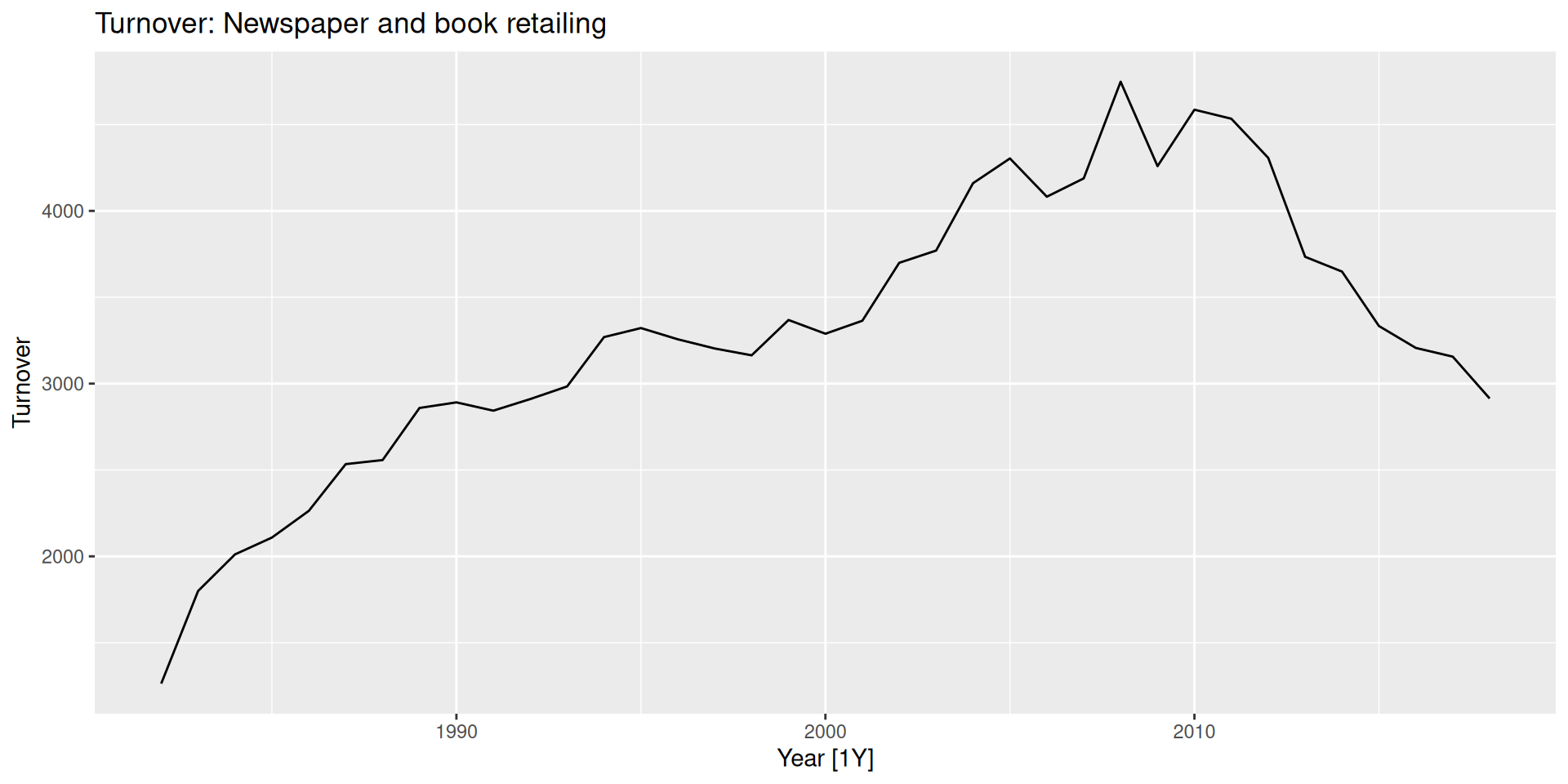
Inflation adjustment example

Inflation adjustment example

• Nominal values
• Real values
• Nominal vs. Real values

aus_economy <- global_economy |>
  filter(Code == "AUS")


print_retail <- print_retail |> 
  left_join(aus_economy, by = "Year") |>
  mutate(Adjusted_turnover = Turnover / CPI) 

Time Series Decomposition

Types of Decompositions

A decomposition splits the time series into its underlying components:

• Trend-cycle
• Seasonal pattern(s)

And what’s left of it we simply call it a “remainder component”.

In general, there are two types of decompositions:

Additive decomposition

\[ y_t = T_t + S_t + R_t \]

Multiplicative decomposition

\[ y_t = T_t \times S_t \times R_t \\ \]

• Which one should you use?

• If the seasonal variation is roughly constant over time, use an additive decomposition.
• If the seasonal variation increases or decreases with the level of the series, use a multiplicative decomposition.
• If you’re unsure, you can try both and see which one provides a better fit.

A multiplicative decomposition is equivalent to an additive decomposition of the log-transformed series:

\[ y_t = T_t \times S_t \times R_t \]

is equivalent to

\[ \log(y_t) = \log(T_t) + \log(S_t) + \log(R_t) \]

Seasonally adjusted series

One use of decomposition is to obtain a seasonally adjusted series, which is the original series with the seasonal component removed.

Seasonally adjusted series can be useful for: - Identifying and analyzing the trend-cycle component without the influence of seasonal fluctuations. - Making comparisons across different time periods without seasonal effects.

• For an additive decomposition, the seasonally adjusted series is given by: \[ y_t - S_t \]
• For a multiplicative decomposition, the seasonally adjusted series is given by: \[ \frac{y_t}{S_t} \]

Classical decomposition

In a classical decomposition, the trend-cycle component is estimated using a moving average. Then, the seasonal component is estimated by averaging the detrended values for each season. Finally, the remainder component is obtained by subtracting the trend-cycle and seasonal components from the original series.

An \(m\) order moving average is given by:

\[ \hat{T}_{t}=\frac{1}{m} \sum_{j=-k}^{k} y_{t+j} \]

where \(k = (m-1)/2\)³.

Example of a classical decomposition

mexretail

Example of a classical decomposition

mexretail |> 
  model()

Example of a classical decomposition

mexretail |> 
  model(
    classical = classical_decomposition() 
  )

Example of a classical decomposition

mexretail |> 
  model(
    classical = classical_decomposition(y, type = "additive") 
  )

Example of a classical decomposition

mexretail |> 
  model(
    classical = classical_decomposition(y, type = "additive") 
  ) |> 
  components()

Example of a classical decomposition

Example of a classical decomposition

Example of a classical decomposition

mexretail_dcmp <- mexretail |>
  model(
    classical = classical_decomposition(y, type = "additive")
  ) |> 
  components()

mexretail_dcmp

1

We start with our original tsibble.

2

Inside the model() function, we specify the type of models we want to use.

3

In any model used, the first thing we need to specify is our forecast variable. Then, depending on the model used, we can specify additional parameters. The model() function yields a mable⁴, which is a table that contains the fitted models for each time series in the tsibble.

4

The components() function is used to extract the components of the decomposition (trend-cycle, seasonal, and remainder) from the fitted models in the mable. It also provides the seasonally adjusted series.

5

Finally, we store the result.

Example of a classical decomposition

mexretail_dcmp |> 
  autoplot()

Problems of using a Classical decomposition

Problems of using a Classical decomposition

• The trend-cycle component is not estimated at the beginning and end of the series. This can be problematic if you want to forecast the series.
• It also tends to over-smooth rises and falls.
• It assumes that the seasonal component is constant over time, which may not be the case in many real-world scenarios.
• It is not robust to outliers, which can significantly affect the estimates of the components.

Warning

It is not recommended to use classical decomposition for forecasting because of these issues.

STL decomposition

STL decomposition

STL (Seasonal and Trend decomposition using Loess) is a more advanced method for decomposing time series data⁵. It uses locally weighted regression (loess) to estimate the trend-cycle and seasonal components. STL is more flexible than classical decomposition and can handle changes in the seasonal component over time.

• It can handle any type of seasonality (not just fixed periods).
• It can handle changes in the seasonal component over time.
• It is robust to outliers.
• It can be used for forecasting.
• It provides a way to control the smoothness of the trend and seasonal components through parameters.

• STL cannot automatically handle calendar or holiday variations.

• It only provides methods for additive models. If your data has multiplicative seasonality, you should log-transform the data before applying STL.

STL in R using fable

mexretail_stl <- mexretail |>                                
  model(                                                      
    stl = STL(y)
  )

STL in R using fable

mexretail_stl <- mexretail |>                                
  model(                                                      
    stl = STL(y ~ trend(window = NULL))
  )

STL in R using fable

mexretail_stl <- mexretail |>                                
  model(                                                      
    stl = STL(y ~ trend()) 
  )

STL in R using fable

STL in R using fable

The code is basically the same as for the classical decomposition. We just need to change the model used inside the model() function.

mexretail |>                                
  model(                                                      
    stl = STL(y ~
                trend(window = NULL) +
                season(window = "periodic"),
              robust = TRUE)
  ) |> 
  components() |> 
  autoplot()

1

Inside the STL() function, we can specify the formula for the decomposition, or don’t specify it at all. See ?STL for more details.

2

The trend() function is used to specify the trend component of the decomposition. The window argument controls the smoothness of the trend component. A larger window results in a smoother trend.

3

The season() function is used to specify the seasonal component of the decomposition. The window argument controls the smoothness of the seasonal component. Setting it to “periodic” means that the seasonal component will be fixed over time.

4

The robust argument, when set to TRUE, makes the STL decomposition more robust to outliers in the data, so the effect of such values is sent to the residual component.

Writing formulas in R

In R, we use “\(\sim\)” instead of “\(=\)” in formula specification, i.e., \(y \sim mx + b\).

Footnotes

1. A time series can have multiple seasonal patterns.

2. They usually last at least 2 years.

3. In R, you can compute any moving average by using the slider::slide_dbl() function.

4. short for “model table”

5. There are other decomposition methods primarily used by official statistics agencies, such as X-11, X-12-ARIMA, and TRAMO/SEATS. However, these methods are not as widely used in the forecasting community as STL. For more on these, see this.